A guide to flowcharts using my Gmisc package. The image is CC by Michael Staats.

A flowchart is a type of diagram that represents a workflow or process. The building blocks are boxes and the arrows that connect them. If you have submitted any research paper the last 10 years you have almost inevitably been asked to produce a flowchart on how you generated your data. While there are excellent click-and-draw tools I have always found it to be much nicer to code my charts. In this post I will go through some of the abilities in my Gmisc package that makes this process smoother.

Main example

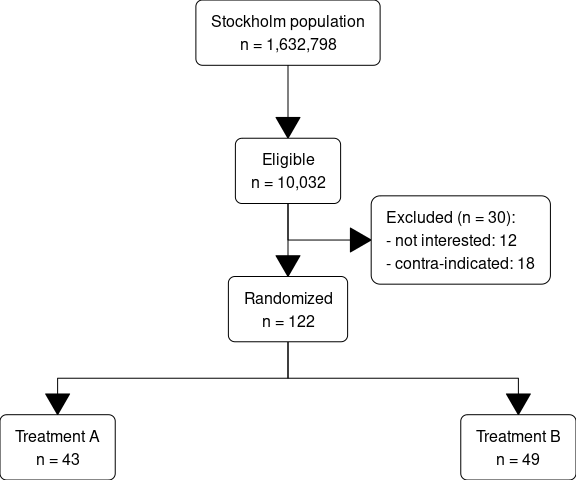
Lets start with the end result when you use Gmisc the boxGrob() with connectGrob() so that you know if you should continue to read.

the code for this is in the vignette, a slightly adapted version looks like this:

library(Gmisc)
library(magrittr)
library(glue)
 
# The key boxes that we want to plot
org_cohort <- boxGrob(glue("Stockholm population",
                           "n = {pop}",
                           pop = txtInt(1632798),
                           .sep = "\n"))
eligible <- boxGrob(glue("Eligible",
                          "n = {pop}",
                           pop = txtInt(10032),
                           .sep = "\n"))
included <- boxGrob(glue("Randomized",
                         "n = {incl}",
                         incl = txtInt(122),
                         .sep = "\n"))
grp_a <- boxGrob(glue("Treatment A",
                      "n = {recr}",
                      recr = txtInt(43),
                      .sep = "\n"))
 
grp_b <- boxGrob(glue("Treatment B",
                      "n = {recr}",
                      recr = txtInt(122 - 43 - 30),
                      .sep = "\n"))
 
excluded <- boxGrob(glue("Excluded (n = {tot}):",
                         " - not interested: {uninterested}",
                         " - contra-indicated: {contra}",
                         tot = 30,
                         uninterested = 12,
                         contra = 30 - 12,
                         .sep = "\n"),
                    just = "left")
 
# Move boxes to where we want them
vert <- spreadVertical(org_cohort,
                       eligible = eligible,
                       included = included,
                       grps = grp_a)
grps <- alignVertical(reference = vert$grps,
                      grp_a, grp_b) %>%
  spreadHorizontal()
vert$grps <- NULL
 
y <- coords(vert$included)$top +
  distance(vert$eligible, vert$included, half = TRUE, center = FALSE)
excluded <- moveBox(excluded,
                    x = .8,
                    y = y)
 
# Connect vertical arrows, skip last box
for (i in 1:(length(vert) - 1)) {
  connectGrob(vert[[i]], vert[[i + 1]], type = "vert") %>%
    print
}
 
# Connnect included to the two last boxes
connectGrob(vert$included, grps[[1]], type = "N")
connectGrob(vert$included, grps[[2]], type = "N")
 
# Add a connection to the exclusions
connectGrob(vert$eligible, excluded, type = "L")
 
# Print boxes
vert
grps
excluded

Example breakdown

There is a lot happening and it may seem overwhelming but it we break it down to smaller chunks it probably makes more sense.

Packages

The first section is just the packages that I use, and apart from the Gmisc package with the main functions I have magrittr that is just for the %>% pipe, and the glue that is convenient for the text generation that allows us to use interpreted string literals that have become standard tooling in many languages (e.g. JavaSript and Python).

Basic boxGrob() calls

After loading the packages we create each box that we want to output. Note that we save each box into a variable:

org_cohort <- boxGrob(glue("Stockholm population",
                           "n = {pop}",
                           pop = txtInt(1632798),
                           .sep = "\n"))

This avoids plotting the box which is the default action when print is called (R does calls print on any object that is outputted to the terminal). By storing the box in a variable we can use this for manipulating the box prior to output. If we would have written as below:

boxGrob(glue("Stockholm population",
             "n = {pop}",
             pop = txtInt(1632798),
             .sep = "\n"))

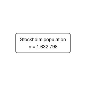
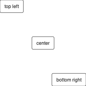
Note that the box is generated in the middle of the image (also known as the main viewport in the grid system). We can choose how to place the box by specifying the position parameters.

boxGrob("top left", y = 1, x = 0, bjust = c(0, 1))
boxGrob("center", y = 0.5, x = 0.5, bjust = c(0.5, 0.5))
boxGrob("bottom right", y = 0, x = 1, bjust = c(1, 0))

Spreading and moving the boxes

While we can position the boxes exactly where we want, I have found it even more useful to move them relative to the available space. The section below does exactly this.

vert <- spreadVertical(org_cohort,
                       eligible = eligible,
                       included = included,
                       grps = grp_a)
grps <- alignVertical(reference = vert$grps,
                      grp_a, grp_b) %>%
  spreadHorizontal()
vert$grps <- NULL
 
excluded <- moveBox(excluded,
                    x = .8,
                    y = coords(vert$included)$top + distance(vert$eligible, vert$included, half = TRUE, center = FALSE))

The spreadVertical() takes each element and calculates the position of each where the first is aligned at the top while the bottom is aligned at the bottom. The elements in between are then spread evenly throughout the available to space. There are some options on how to spread the objects, the default is to have the space between the boxes to be identical but there is also the option of having the center of each box to be evenly spread (see the .type parameter).

The alignVertical() aligns the elements in relation to the reference object. In this case we chose to find the bottom alignment using a “fake” grp_a box. As we only have this box so that we can use it for future alignment we dopr the box with vert$grps <- NULL.

Note that all of the align/spread functions return a list with the boxes in the new positions (if you print the original boxes they will not have moved). Thus make sure you print the returned elements if you want to see the objects, just as we do at the end of the code block.

vert
grps
excluded

Moving a box

In the example we want the exclusions to be equally spaced between the eligible and included which we can do using moveBox() that allows us to change any of the coordinates for the original box. Just as previously, we save the box onto the original variable or the box would appear not to have moved once we try to print it.

Here we also make use of the coords() function that gives us access to the coordinates of a box and the distance() that gives us the distance between boxes (the center = FALSE is for retrieving the distance between the boxes edges and not from the center point).

y <- coords(vert$included)$top +
  distance(vert$eligible, vert$included, half = TRUE, center = FALSE)
excluded <- moveBox(excluded,
                    x = .8,
                    y = y)

Generating the connecting arrows

Once we are done with positioning all the boxes we need to connect them using the arrows using the connectGrob(). The function accepts two boxes and draws a line between them. The appearance
of the line is decided by the type argument. My apologies it the allowed arguments "vertical", "horizontal", "L", "-", "Z", "N" are not super intuitive, finding good names is hard. Feel free to suggest better options/explanations. Anyway, below we simply loop through them all and plot the arrows using print(). Note that we only need to call print() within the for loop as the others are automatically printed.

for (i in 1:(length(vert) - 1)) {
  connectGrob(vert[[i]], vert[[i + 1]], type = "vert") %>%
    print
}
connectGrob(vert$included, grps[[1]], type = "N")
connectGrob(vert$included, grps[[2]], type = "N")
 
connectGrob(vert$eligible, excluded, type = "L")

Short summary

So the basic workflow is

• generate boxes,
• position them,
• connect arrows to them, and
• print

Practical tips

I have found that generating the boxes simultaneous to when I actually exclude the examples in my data set keeps the risk of invalid counts to a minimum. Sometimes I generate a list that I later convert to a flowchart, but the principle is the same - make sure the graph is closely related to your data.

If you want to style your boxes you can set the options(boxGrobTxt=..., boxGrob=...) and all boxes will have the same styling. The fancy boxPropGrob() allows you to show data splits and has even more options that you may want to check out, although usually you don't have more than one boxPropGrob().