Few of us can resist chocolate, but the real question is: should we even try to resist it? The image is CC by Tasumi1968.
As a dark chocolate addict I was relieved to see Messerli’s ecological study on chocolate consumption and the relation to the Nobel prize. By scraping various on-line sources he made a robust case for that increased chocolate consumption correlates to the number of Nobel prizes. Combined with that it might have positive impact on blood pressure, the evidence is strong enough for me to avoid changing any habits, at least over Christmas 🙂
- F. H. Messerli, “Chocolate Consumption, Cognitive Function, and Nobel Laureates,” New England Journal of Medicine, vol. 367, no. 16, pp. 1562–1564, 2012.
- K. Ried, T. Sullivan, P. Fakler, O. R. Frank, and N. P. Stocks, “Does chocolate reduce blood pressure? A meta-analysis,” BMC Medicine, vol. 8, no. 1, p. 39, 2010.
Tutorial: Scraping the chocolate data with R
Inspired by Messerli’s article I decided to look into how to repeat the analysis in R.
We will start by getting Nobel prizes per country using readHTMLTable() from the XML package, followed by some data cleaning.
library(XML)
theurl <- "http://en.wikipedia.org/wiki/List_of_countries_by_Nobel_laureates_per_capita"
tables <- readHTMLTable(theurl)

nobel_prizes <- tables[[2]]
# Clean column names
colnames(nobel_prizes) <-
  gsub(" ", "_",
       gsub("(/|\\[[0-9]+\\])", "",
            gsub("\n", " ", colnames(nobel_prizes))
        )
    )

# Delete those that aren't countries and thus lack rank
nobel_prizes$Rank <- as.numeric(as.character(nobel_prizes$Rank))
nobel_prizes <- subset(nobel_prizes, is.na(Rank) == FALSE)

# Clean the country names
nobel_prizes$Country <-
  gsub("[^a-zA-Z ]", "", nobel_prizes$Country)

# Clean the loriates variable
nobel_prizes$Laureates_10_million <-
  as.numeric(as.character(nobel_prizes$Laureates_10_million))
Chocolate data
We need to set Swiss' consumption by hand since it's only specified in the article.
nobel_prizes$Chocolate_consumption <- NA
# http://www.chocosuisse.ch/web/chocosuisse/en/documentation/faq.html
nobel_prizes$Chocolate_consumption[nobel_prizes$Country == "Switzerland"] <- 11.9
The next part is slightly trickier since we need to translate German country names to match the Nobel prize data.
# Translation from German to English
theurl <- "http://german.about.com/library/blnation_index.htm"

tables <- readHTMLTable(theurl)

translate_german <- tables[[1]]
translate_german <- translate_german[3:NROW(translate_german), 1:2]
colnames(translate_german) <- c("English", "German")
translate_german$German <-
    gsub("([ ]+(f|pl)\\.$|\\([[:alnum:] -]+\\))", "", translate_german$German)
Now lets go for the actual data.
# Get the consumption from a German list
theurl <- "http://www.theobroma-cacao.de/wissen/wirtschaft/international/konsum"

tables <- readHTMLTable(theurl)

german_chocolate_data <- tables[[1]][2:NROW(tables[[1]]), ]
names(german_chocolate_data) <- c("Country", "Chocolate_consumption")
german_chocolate_data$Country <-
    gsub("([ ]+f\\.$|\\([[:alnum:] -]+\\))", "", german_chocolate_data$Country)

library(sqldf)

sql <- paste0("SELECT gc.*, tg.English as Country_en",
              " FROM german_chocolate_data AS gc",
              " LEFT JOIN translate_german AS tg",
              " ON gc.Country = tg.German",
              " OR gc.Country = tg.English")
german_chocolate_data <- sqldf(sql)

german_chocolate_data$Country <-
    ifelse(is.na(german_chocolate_data$Country_en),
    german_chocolate_data$Country,
    german_chocolate_data$Country_en)

german_chocolate_data$Country_en <- NULL
german_chocolate_data$Chocolate_consumption_tr <- NA
for (i in 1:NROW(german_chocolate_data)) {
    number <- as.character(german_chocolate_data$Chocolate_consumption[i])
    if (length(number) > 0) {
        m <- regexpr("^([0-9]+,[0-9]+)", number)
        if (m > 0) {
            german_chocolate_data$Chocolate_consumption_tr[i] <-
                as.numeric(
                    sub(",", ".", regmatches(number, m))
                )
        } else {
            m <- regexpr("\\(([0-9]+,[0-9]+)", number)

            if (m > 0)
                german_chocolate_data$Chocolate_consumption_tr[i] <-
                    as.numeric(
                        sub("\\(", "",
                            sub(",", ".", regmatches(number, m))
                        )
                    )
        }
    }
}

sql <- paste0("SELECT np.*, gp.Chocolate_consumption_tr AS choc",
              " FROM nobel_prizes AS np",
              " LEFT JOIN german_chocolate_data AS gp",
              " ON gp.Country = np.Country")
nobel_prizes <- sqldf(sql)
Unfortunately the the Caobisco referenced PDF can't be found :-(. Although it might be for the best since PDF data is very difficult to mine. One option could be to use the PDF to Word converter and hope for it to return a readable table.
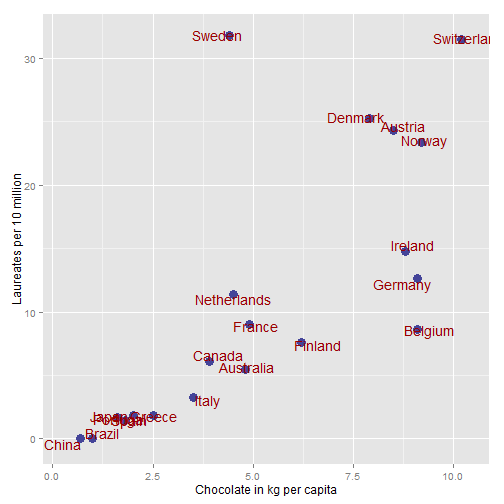
This leaves us with 20 countries that have chocolate data. Lets plot it:
library(ggplot2)
ggplot(data = subset(nobel_prizes, is.na(choc) == FALSE), aes(x = choc, y = Laureates_10_million)) +
    ylab("Laureates per 10 million") + xlab("Chocolate in kg per capita") +
    geom_point(size = 4, colour = "#444499") + geom_text(aes(label = Country),
    size = 5, position = position_jitter(width = 0.5, height = 0.5), colour = "#990000")
BMI - adding something new to the dataset
Now just to add some more fun to the data, lets look at obesity. I've found a simple table with male obesity available for scraping after a quick Google search (yes I know, it's only men, if you know a better table please post a comment and I'll change it).
# Percentage of males with a BMI > 25 kg/m2
tables <- readHTMLTable("http://www.oecd-ilibrary.org/sites/ovob-ml-table-2012-2-en/index.html;jsessionid=18wcxgabwn3ou.x-oecd-live-02?contentType=/ns/KeyTable,/ns/StatisticalPublication&itemId=/content/table/20758480-table16&containerItemId=/content/tablecollection/20758480&accessItemIds=&mimeType=text/html")

ob <- tables[[1]]
ob[, 2] <- as.character(ob[, 2])
ob <- apply(ob, FUN = as.character, MARGIN = 2)
ob <- ob[, 2:NCOL(ob)]
ob <- ob[4:NROW(ob), ]

last_obesitas <- apply(apply(ob[, 2:NCOL(ob)], FUN = as.numeric, MARGIN = 2),
    MARGIN = 1, FUN = function(x) {
        if (any(is.na(x) == FALSE))
            return(x[max(which(is.na(x) == FALSE))]) else return(NA)
    })

ob <- data.frame(Country = ob[, 1], last_obesitas = last_obesitas)
ob <- subset(ob, is.na(last_obesitas) == FALSE)

sql <- paste0("SELECT np.*, ob.last_obesitas AS obesitas",
              " FROM nobel_prizes AS np",
              " LEFT JOIN ob", " ON ob.Country = np.Country")
nobel_prizes <- sqldf(sql)
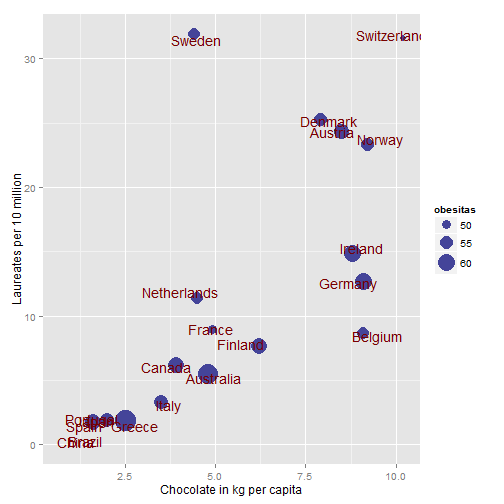
Now lets add it to our amazing plot:
ggplot(data = subset(nobel_prizes, is.na(choc) == FALSE), aes(x = choc, y = Laureates_10_million)) +
    ylab("Laureates per 10 million") + xlab("Chocolate in kg per capita") +
    geom_point(aes(size = obesitas), colour = "#444499") + scale_size(range = c(3,
    10)) + geom_text(aes(label = Country), size = 5, position = position_jitter(width = 0.5,
    height = 0.5), colour = "#770000")

A ggplot with the chocolate consumption and Nobel laureates with the obesity as size of the dots. It would be fun to add the country flags as in the original article. The names tend to get a little crowded, but I haven't figured that one out yet... Ideally it would be something like the bus svg image in Murrel & Ly's article in the R journal
The model
Now if you want to compare our results to the original article you can find the model output below.
fit <- lm(Laureates_10_million ~ choc, data = nobel_prizes)
summary(fit)
## Call:
## lm(formula = Laureates_10_million ~ choc, data = nobel_prizes)
##
## Residuals:
## Min 1Q Median 3Q Max
## -11.94 -3.87 -1.28 2.16 22.77
##
## Coefficients:
## Estimate Std. Error t value Pr(>|t|)
## (Intercept) -1.657 3.283 -0.50 0.61995
## choc 2.442 0.541 4.51 0.00027 ***
## ---
## Signif. codes: 0 '***' 0.001 '**' 0.01 '*' 0.05 '.' 0.1 ' ' 1
##
## Residual standard error: 7.45 on 18 degrees of freedom
## (51 observations deleted due to missingness)
## Multiple R-squared: 0.531, Adjusted R-squared: 0.505
## F-statistic: 20.4 on 1 and 18 DF, p-value: 0.000269


Could you please post the resultant dataset?
Sure, did you have trouble getting the code to run? Here’s a dput:
[code]structure(list(Rank = c(1, 2, 3, 4, 5, 6, 7, 8, 9, 10, 11, 12,
13, 14, 15, 16, 17, 18, 19, 20, 21, 22, 23, 24, 25, 26, 27, 28,
29, 30, 31, 32, 33, 34, 35, 36, 37, 38, 39, 40, 41, 42, 43, 44,
45, 46, 47, 48, 49, 50, 51, 52, 53, 54, 55, 56, 57, 58, 59, 60,
61, 62, 63, 64, 65, 66, 67, 68, 69, 70, 71), Country = c("Saint Lucia",
"Luxembourg", "Iceland", "Sweden", "Switzerland", "Denmark",
"Austria", "Norway", "United Kingdom", "TimorLeste", "Ireland",
"Israel", "Germany", "Netherlands", "United States", "Hungary",
"France", "Cyprus", "Belgium", "Trinidad and Tobago", "Finland",
"New Zealand", "Canada", "Australia", "Bosnia and Herzegovina",
"Liberia", "Slovenia", "Czech Republic", "Macedonia", "Latvia",
"Italy", "Poland", "Lithuania", "Croatia", "Costa Rica", "Greece",
"Portugal", "South Africa", "Spain", "Russia", "Japan", "Bulgaria",
"Guatemala", "Romania", "Argentina", "Chile", "Azerbaijan", "Belarus",
"Algeria", "Egypt", "Taiwan", "Ghana", "Yemen", "Venezuela",
"Peru", "Morocco", "Mexico", "Iran", "Kenya", "Ukraine", "Colombia",
"Korea South", "Burma", "Turkey", "Vietnam", "India", "Bangladesh",
"China", "Nigeria", "Pakistan", "Brazil"), Nobel_laureates = structure(c(9L,
9L, 1L, 14L, 13L, 7L, 10L, 4L, 5L, 9L, 21L, 2L, 3L, 8L, 16L,
24L, 20L, 1L, 24L, 1L, 17L, 15L, 11L, 6L, 9L, 9L, 1L, 19L, 1L,
1L, 10L, 6L, 1L, 1L, 1L, 9L, 9L, 24L, 22L, 12L, 8L, 1L, 9L, 15L,
19L, 9L, 1L, 1L, 9L, 17L, 1L, 1L, 1L, 1L, 1L, 1L, 15L, 9L, 1L,
1L, 1L, 1L, 1L, 1L, 1L, 24L, 1L, 22L, 1L, 1L, 1L), .Label = c("1",
"10", "103", "11", "119", "12", "14", "19", "2", "20", "21",
"23", "25", "29", "3", "338", "4", "466", "5", "59", "7", "8",
"839", "9"), class = "factor"), Population__2012_ = c("162,178",
"509,074", "313,183", "9,103,788", "7,925,517", "5,543,453",
"8,219,743", "4,707,270", "63,047,162", "1,143,667", "4,722,028",
"7,590,758", "81,305,856", "16,730,632", "314,976,000", "9,958,453",
"65,630,692", "1,138,071", "10,438,353", "1,226,383", "5,262,930",
"4,327,944", "34,300,083", "22,015,576", "3,879,296", "3,887,886",
"1,996,617", "10,177,300", "2,082,370", "2,191,580", "61,261,254",
"38,415,284", "3,525,761", "4,480,043", "4,636,348", "10,767,827",
"10,781,459", "48,810,427", "47,042,984", "142,517,670", "127,368,088",
"7,037,935", "14,099,032", "21,848,504", "42,192,494", "17,067,369",
"9,493,600", "9,643,566", "37,367,226", "83,688,164", "23,234,936",
"24,652,402", "24,771,809", "28,047,938", "29,549,517", "32,309,239",
"114,975,406", "78,868,711", "43,013,341", "44,854,065", "45,239,079",
"48,860,500", "54,584,650", "79,749,461", "91,519,289", "1,205,073,612",
"161,083,804", "1,343,239,923", "170,123,740", "190,291,129",
"199,321,413"), Laureates_10_million = c(123.321, 39.287, 31.93,
31.855, 31.544, 25.255, 24.332, 23.368, 18.875, 17.488, 14.824,
13.174, 12.668, 11.356, 10.731, 9.038, 8.99, 8.787, 8.622, 8.154,
7.6, 6.932, 6.122, 5.451, 5.156, 5.144, 5.008, 4.913, 4.802,
4.563, 3.265, 3.124, 2.836, 2.232, 2.157, 1.857, 1.855, 1.844,
1.701, 1.614, 1.492, 1.421, 1.419, 1.373, 1.185, 1.172, 1.053,
1.037, 0.535, 0.478, 0.43, 0.406, 0.404, 0.357, 0.338, 0.31,
0.261, 0.254, 0.232, 0.223, 0.221, 0.205, 0.183, 0.125, 0.109,
0.075, 0.062, 0.06, 0.059, 0.053, 0.05), Chocolate_consumption = c(NA,
NA, NA, NA, 11.9, NA, NA, NA, NA, NA, NA, NA, NA, NA, NA, NA,
NA, NA, NA, NA, NA, NA, NA, NA, NA, NA, NA, NA, NA, NA, NA, NA,
NA, NA, NA, NA, NA, NA, NA, NA, NA, NA, NA, NA, NA, NA, NA, NA,
NA, NA, NA, NA, NA, NA, NA, NA, NA, NA, NA, NA, NA, NA, NA, NA,
NA, NA, NA, NA, NA, NA, NA), choc = c(NA, NA, NA, 4.4, 10.2,
7.9, 8.5, 9.2, NA, NA, 8.8, NA, 9.1, 4.5, NA, NA, 4.9, NA, 9.1,
NA, 6.2, NA, 3.9, 4.8, NA, NA, NA, NA, NA, NA, 3.5, NA, NA, NA,
NA, 2.5, 2, NA, 1.6, NA, 1.8, NA, NA, NA, NA, NA, NA, NA, NA,
NA, NA, NA, NA, NA, NA, NA, NA, NA, NA, NA, NA, NA, NA, NA, NA,
NA, NA, 0.7, NA, NA, 1), obesitas = c(NA, NA, 66.7, 53.6, 46.3,
54.3, 56.9, 55, NA, NA, 59, NA, 60.1, 53.6, 70.2, 59.4, 49.9,
NA, 53.7, NA, 57.9, NA, 58.9, 63.3, NA, NA, 64.9, 62.5, NA, NA,
55.5, 61.4, NA, NA, NA, 64.9, 56, NA, 58.6, NA, NA, NA, NA, NA,
NA, 50.1, NA, NA, NA, NA, NA, NA, NA, NA, NA, NA, NA, NA, NA,
NA, NA, NA, NA, 50.4, NA, NA, NA, NA, NA, NA, NA)), .Names = c("Rank",
"Country", "Nobel_laureates", "Population__2012_", "Laureates_10_million",
"Chocolate_consumption", "choc", "obesitas"), row.names = c(NA,
71L), class = "data.frame")[/code]