Putting all the pieces together can be challenging both for surgeons and researchers. The image is CC by Zac Peckler

Fast-track publishing using knitr is a short series on how I use knitr to speedup publishing in my research. There has been plenty of feedback and interest for the series, and in this post I would like to provide (1) a brief summary and (2) an example showing how to put all the pieces together.

The series consists out of five posts:

• First post – an intro motivating knitr in writing your manuscript and a comparison of knitr to Word options.
• Second post – setting up a .RProfile and using a custom.css file.
• Third post – getting your plots the way you want.
• Fourth post – generating tables.
• Fifth post – summary and example (current post).

Summary

The main idea of fast-track publishing is taking the reproducible research approach one step further by looking how we can combine the ideas of reproducible research with good layout, handling images, table generation, and MS Word-integration. The aim of each is:

• Layout: if you stick to good layout practices your co-authors and reviewers will most likely have a faster response time.
• Images: submitting and sharing images should be a no-brainer.
• Tables: tables contain a lot of information and a lot of layout, having a good-looking standard solution saves you time.
• MS Word integration: tracking changes and adding comments directly is vital when working on your manuscript. I dream of being able to share my knitr Rmd-files with my co-authors, unfortunately sharing a raw document with code is not an option.

My current way of doing this is by using knitr markdown with a custom.css together with some functions from my Gmisc-package. As some have suggested, interesting alternatives are Pandoc and R2DOCX, although I’ve found tables to be less flexible with those.

Lastly, I currently do not recommend writing your full document in knitr; focus on the data-specifics such as parts of the methods sections and the results section. You will otherwise spend too much time manually changing references and there is currently no simple way to get the rich bibliography types that Zotero, Endnote, and Mendeley provide.

Fast-track example

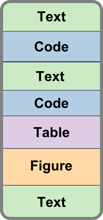
A knitr document mixes four different elements: plain text, code, tables, and figures. This is why it is called weaving/knitting a document. Below you can see the general idea of the document structure:

To separate code from text, knitr markdown uses chunks; ```{r} indices start of a chunk while ``` indicates the end. To work nicely with RStudio you also need to remember to save your file with a .Rmd file ending, otherwise RStudio doesn’t know that it is a knitr markdown document.

The actual example (sorry, couldn’t get the syntax highlighting to work):

```{r Data_prep, echo=FALSE, message=FALSE, warning=FALSE}
# Moved this outside the document for easy of reading
# I often have those sections in here
source("Setup_and_munge.R")
```

```{r Versions}
info <- sessionInfo()
r_ver <- paste(info$R.version$major, info$R.version$minor, sep=".")
```

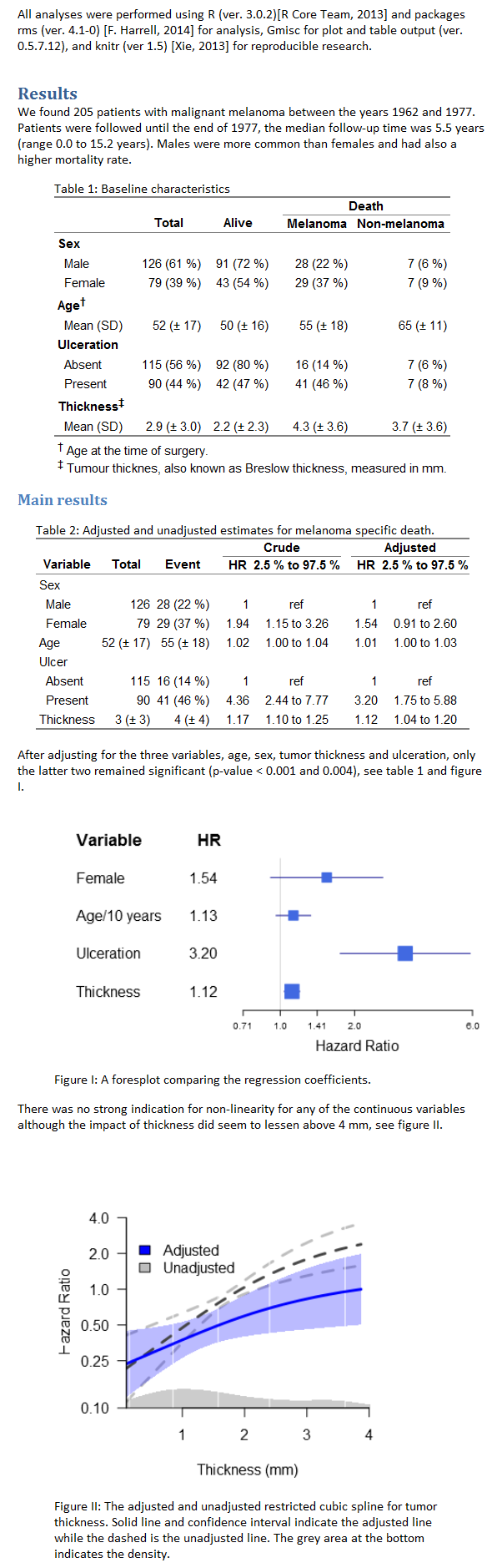
All analyses were performed using R (ver. `r r_ver`)[R Core Team, 2013] 
and packages rms (ver. `r info$otherPkgs$rms$Version`) [F. Harrell, 2014] 
for analysis, Gmisc for plot and table output (ver. `r info$otherPkgs$Gmisc$Version`), 
and knitr (ver `r info$otherPkgs$knitr$Version`) [Xie, 2013] for reproducible research.

Results
=======

We found `r nrow(melanoma)` patients with malignant melanoma between the years 
`r paste(range(melanoma$year), collapse=" and ")`. Patients were followed until 
the end of 1977, the median follow-up time was `r sprintf("%.1f", median(melanoma$time_years))` 
years (range `r paste(sprintf("%.1f", range(melanoma$time_years)), collapse=" to ")` years). 
Males were more common than females and had also a higher mortality rate.

```{r Table1, results='asis', cache=FALSE}
table_data <- list()
getT1Stat <- function(varname, digits=0){
  getDescriptionStatsBy(melanoma[, varname], melanoma$status, 
                        add_total_col=TRUE,
                        show_all_values=TRUE, 
                        hrzl_prop=TRUE,
                        statistics=FALSE, 
                        html=TRUE, 
                        digits=digits)
}

# Get the basic stats
table_data[["Sex"]] <- getT1Stat("sex")
table_data[["Age†"]] <- getT1Stat("age")
table_data[["Ulceration"]] <- getT1Stat("ulcer")
table_data[["Thickness‡"]] <- getT1Stat("thickness", digits=1)

# Now merge everything into a matrix
# and create the rgroup & n.rgroup variabels
rgroup <- c()
n.rgroup <- c()
output_data <- NULL
for (varlabel in names(table_data)){
  output_data <- rbind(output_data, table_data[[varlabel]])
  rgroup <- c(rgroup, varlabel)
  n.rgroup <- c(n.rgroup, nrow(table_data[[varlabel]]))
}

# Add a column spanner for the death columns
cgroup <- c("", "Death")
n.cgroup <- c(2, 2)
colnames(output_data) <- gsub("[ ]*death", "", colnames(output_data))

htmlTable(output_data, align="rrrr",
          rgroup=rgroup, n.rgroup=n.rgroup, 
          rgroupCSSseparator="", 
          cgroup = cgroup,
          n.cgroup = n.cgroup,
          rowlabel="", 
          caption="Baseline characteristics", 
          tfoot=paste0("† Age at the time of surgery.",
                       " 
‡ Tumour thicknes,",
                       " also known as Breslow thickness, measured in mm."), 
          ctable=TRUE)
```

Main results
------------

```{r C_and_A, results='asis'}
# Setup needed for the rms coxph wrapper
ddist <- datadist(melanoma)
options(datadist = "ddist")

# Do the cox regression model 
# for melanoma specific death
msurv <- Surv(melanoma$time_years, melanoma$status=="Melanoma death")
fit <- cph(msurv ~ sex + age + ulcer + thickness, data=melanoma)

# Print the model
printCrudeAndAdjustedModel(fit, desc_digits=0,
                           caption="Adjusted and unadjusted estimates for melanoma specific death.",
                           desc_column=TRUE,
                           add_references=TRUE, 
                           ctable=TRUE)

pvalues <- 
  1 - pchisq(coef(fit)^2/diag(vcov(fit)), df=1)
```

After adjusting for the three variables, age, sex, tumor thickness
 and ulceration, only the latter two remained significant (p-value 
`r pvalueFormatter(pvalues["ulcer=Present"], sig.limit=10^-3)` and
`r pvalueFormatter(pvalues["thickness"], sig.limit=10^-3)`), 
see table `r as.numeric(options("table_counter"))-1` and 
figure `r getNextFigureNo()`.

```{r Regression_forestplot, fig.height=3, fig.width=5, fig.cap="A foresplot comparing the regression coefficients."}
# I've adjusted the coefficient for age to be by 
forestplotRegrObj(update(fit, .~.-age+I(age/10)), 
                  order.regexps=c("Female", "age", "ulc", "thi"),
                  box.default.size=.25, xlog=TRUE,
                  new_page=TRUE, clip=c(.5, 6), rowname.fn=function(x){
  if (grepl("Female", x))
    return("Female")
  
  if (grepl("Present", x))
    return("Ulceration")
  
  if (grepl("age", x))
    return("Age/10 years")

  return(capitalize(x))
})
```

There was no strong indication for non-linearity for any of the 
continuous variables although the impact of thickness did 
seem to lessen above 4 mm, see figure `r getNextFigureNo()`.

```{r spline_plot, fig.cap=plotHR_cap}
plotHR_cap = paste0("The adjusted and unadjusted restricted cubic spline",
                    " for tumor thickness. Solid line and confidence interval",
                    " indicate the adjusted line while the dashed is",
                    " the unadjusted line. The grey area at ",
                    " the bottom indicates the density.")
# Generate adjusted and anuadjusted regression models
rcs_fit <- update(fit, .~.-thickness+rcs(thickness, 3))
rcs_fit_ua <- update(fit, .~+rcs(thickness, 3))

# Make sure the axes stay at the exact intended points
par(xaxs="i", yaxs="i")
plotHR(list(rcs_fit, rcs_fit_ua), col.dens="#00000033",
       lty.term=c(1, 2),
       col.term=c("blue", "#444444"), 
       col.se = c("#0000FF44", "grey"),
       polygon_ci=c(TRUE, FALSE),
       term="thickness", 
       xlab="Thickness (mm)", 
       ylim=c(.1, 4), xlim=c(min(melanoma$thickness), 4), 
       plot.bty="l", y.ticks=c(.1, .25, .5, 1, 2, 4))
legend(x=.1, y=1.1, legend=c("Adjusted", "Unadjusted"), fill=c("blue", "grey"), bty="n")
```

The external code for the first chunk:

##################
# Knitr settings #
##################

# Don't set knitr options outside knitr
if ("package:knitr" %in% search()){
  # Set some basic options. You usually do not
  # want your code, messages, warnings etc
  # to show in your actual manuscript
  opts_chunk$set(warning=FALSE, 
                 message=FALSE, 
                 echo=FALSE, 
                 dpi=96,
                 fig.width=4, fig.height=4, # Default figure widths
                 dev="png", dev.args=list(type="cairo"), # The png device
                 # Change to dev="postscript" if you want the EPS-files
                 # for submitting. Also remove the dev.args() as the postscript
                 # doesn't accept the type="cairo" argument.
                 error=FALSE)
  
  # Evaluate the figure caption after the plot
  opts_knit$set(eval.after='fig.cap')
  
  # Avoid including base64_images - this only 
  # works with the .RProfile setup
  options(base64_images = "none")
  
  # Add a figure counter function
  knit_hooks$set(plot = function(x, options) {
    fig_fn = paste0(opts_knit$get("base.url"), 
                    paste(x, collapse = "."))
    
    # Some stuff from the default definition
    fig.cap <- knitr:::.img.cap(options)
    
    # Style and additional options that should be included in the img tag
    style=c("display: block",
            sprintf("margin: %s;",
                    switch(options$fig.align, 
                           left = 'auto auto auto 0', 
                           center = 'auto',
                           right = 'auto 0 auto auto')))
    # Certain arguments may not belong in style, 
    # for instance the width and height are usually
    # outside if the do not have a unit specified
    addon_args = ""
    
    # This is perhaps a little overly complicated prepared 
    # with the loop but it allows for a more out.parameters if necessary
    if (any(grepl("^out.(height|width)", names(options)))){
      on <- names(options)[grep("^out.(height|width)", names(options))]
      for(out_name in on){
        dimName <- substr(out_name, 5, nchar(out_name))
        if (grepl("[0-9]+(em|px|%|pt|pc|in|cm|mm)", out_name))
          style=append(style, paste0(dimName, ": ", options[[out_name]]))
        else if (length(options$out.width) > 0)
          addon_args = paste0(addon_args, dimName, "='", options[[out_name]], "'")
      }
    }
    
    # Add counter if wanted
    fig_number_txt <- ""
    cntr <- getOption("figure_counter", FALSE)
    if (cntr != FALSE){
      if (is.logical(cntr))
        cntr <- 1
      # The figure_counter_str allows for custom 
      # figure text, you may for instance want it in
      # bold: Figure %s:
      # The %s is so that you have the option of setting the
      # counter manually to 1a, 1b, etc if needed
      fig_number_txt <- 
        sprintf(getOption("figure_counter_str", "Figure %s: "), 
                ifelse(getOption("figure_counter_roman", FALSE), 
                       as.character(as.roman(cntr)), as.character(cntr)))
      
      if (is.numeric(cntr))
        options(figure_counter = cntr + 1)
    }
    
    # Put it all together
    paste0("
",
           "
")
  })
  
}

# Use the table counter that the htmlTable() provides
options(table_counter = TRUE)

# Use the figure counter that we declare below
options(figure_counter = TRUE)
# Use roman letters (I, II, III, etc) for figures
options(figure_counter_roman = TRUE)

# Adding the figure number is a little tricky when the format is roman
getNextFigureNo <- function() as.character(as.roman(as.numeric(options("figure_counter"))))

#################
# Load_packages #
#################
library(rms) # I use the cox regression from this package
library(boot) # The melanoma data set is used in this exampe
library(Gmisc) # Stuff I find convenient
library(Greg) # You need to get this from my GitHub see http://gforge.se/Gmisc

##################
# Munge the data #
##################

# Here we go through and setup the variables so that
# they are in the proper format for the actual output

# Load the dataset - usually you would use read.csv
# or something similar
data("melanoma")

# Set time to years instead of days
melanoma$time_years <- 
  melanoma$time / 365.25

# Factor the basic variables that 
# we're interested in
melanoma$status <- 
  factor(melanoma$status, 
         levels=c(2, 1, 3),
         labels=c("Alive", # Reference
                  "Melanoma death", 
                  "Non-melanoma death"))
melanoma$sex <- 
  factor(melanoma$sex,
         labels=c("Male", # Reference
                  "Female"))

melanoma$ulcer <- 
  factor(melanoma$ulcer,
         levels=0:1,
         labels=c("Absent", # Reference
                  "Present"))

Together with the previous custom.css and .Rprofile generate this:

You can find all the files that you need at the FTP-github page.

I hope you enjoyed the series and that you've find it useful. I wish that we would one day have a Word-alternative with track-changes, comments, version-handling etc that would allow true FTP, but until then this is my best alternative. Perhaps the talented people at RStudio can come up with something that fills this void?