

Finding the right curve can be tricky. The image is CC by Martin Gommel.
In my previous post I wrote about the importance of age and why it is a good idea to try avoiding modeling it as a linear variable. In this post I will go through multiple options for (1) modeling non-linear effects in a linear regression setting, (2) benchmark the methods on a real dataset, and (3) look at how the non-linearities actually look. The post is based on the supplement in my article on age and health-related quality of life (HRQoL).
Background
What is linearity?
Wikipedia has an excellent explanation of linearity:
linearity refers to a mathematical relationship or function that can be graphically represented as a straight line
Why do we assume linearity?
Linearity is a common assumption that is made when building a linear regression model. In a linear relation, a continuous variable has the same impact throughout the variable’s span. This makes the estimate is easy to interpret; an increase of one unit gives the corresponding coefficient’s change in the outcome. While this generates simple models with its advantages, it is difficult to believe that nature follows a simple straight line. With todays large data sets I believe that our models should permit non-linear effects.
How do we do non-linearity?
There are plenty of non-linear alternatives that can be used to better find the actual relationships. Most of them rely on converting the single continuous variable into several. The simplest form is when we transform the variable into a polynomial, e.g. instead of having the model:
HRQoL ~ β0 + βage * Age + βsex * Sex
We expand age to also include the age squared:
HRQoL ~ β0 + βage * Age + βage” * Age2 + βsex * Sex
This allows for the line for a bend, unfortunately as we add the squared term the coefficients are more difficult to interpret, and after adding a cubic term, i.e. Age3, it is almost impossible to interpret the coefficients. Due to this difficulty in interpretation I either use the rms::contrast function or the stats::predict in order to illustrate how the variable behaves.
Splines
A frequently used alternative to polynomials are splines. The most basic form of a spline consists of lines that are connected at different “knots”. For instance, a linear spline with 1 knot can assume a V-shape, while 2 knots allow for an N-shaped relationship. The number of knots decide the flexibility of a spline, i.e. more knots allow a more detailed description of the relationship.
The models
The dataset comes from the Swedish Hip Arthroplasty Register‘s excellent PROM database and consists of more than 30,000 patients that have filled out the EQ-5D form both before and after surgery. We will focus on age and its impact on the EQ-5D index and the EQ-VAS one year after total hip replacement surgery. We will control for sex, Charnley class, pre-operative HRQoL, pre-operative pain.
The restricted cubic spline
I’m a big fan of Frank Harrell‘s rms-package so we will start there although we start by splitting the dataset using the caret::createDataPartition. We then need to set the rms::datadist in order for the rms-functions to work as expected:
library(caret)
train_no
Frank Harrell is a proponent of restricted cubic splines, alias natural cubic splines. This is a type of spline that uses cubic terms in the center of the data and restricts the ends to a straight line, preventing the center from distorting the ends, i.e. curling. His rcs() also nicely integrates with the anova in order to check if non-linearity actually exists:
idx_model
gives:
Analysis of Variance          Response: eq5d1

 Factor                                              F      d.f. P
 Age                                                 140.71  2
As we can see the model seems OK for the EQ-5D index, supporting both the non-linearity and the interaction between Charnley class and sex. If we for some reason cannot use the rms-package we can check for linearity by using the splines::ns with two regular models as suggested below:
lm1
gives:
Analysis of Variance Table

Model 1: eq5d1 ~ Age + Sex * Charnley_class + ns(eq5d0, 3) + ns(pain0,
    3)
Model 2: eq5d1 ~ ns(Age, 3) + Sex * Charnley_class + ns(eq5d0, 3) + ns(pain0,
    3)
  Res.Df    RSS Df Sum of Sq      F    Pr(>F)
1  19095 193.01
2  19093 192.66  2   0.35112 17.398 2.825e-08 ***
---
Signif. codes:  0 ‘***’ 0.001 ‘**’ 0.01 ‘*’ 0.05 ‘.’ 0.1 ‘ ’ 1
In order to avoid overfitting we will try to select models based upon the AIC/BIC criteria. The selection is simply finding the lowest value where in general AIC allows slightly more complex models compared to BIC. We will start with finding the optimal number of knots for the EQ-5D index using the AIC:
#' A simple function for updating the formula and extracting
#' the information criteria
#'
#' @param no A number that is used together with the add_var_str
#' @param fit A regression fit that is used for the update
#' @param rm_var The variable that is to be substituted
#' @param add_var_str A sprintf() string that accepts the no
#'  parameter for each update
#' @param ic_fn The information criteria function (AIC/BIC)
getInfCrit
It can be discussed if the model should stop at 3 knots but I chose to continue a little higher as the drop was relatively large between the 4 and 5 knots. This is most likely due to a unfortunate fit for the 4 knots. We could also have motivated a larger number of knots but even with proper visualization these are difficult to interpret. When modeling confounders, such as the preoperative EQ-5D index (eq5d0) and the pre-operative pain (pain0), we may prefer a higher number of knots in order to avoid any residual confounding and we do not need to worry about visualizing/explaining the relations.
Now if we apply the same methodology to the EQ-VAS we get:
vas_model
Now lets do the same for the BIC:
idx_model
B-splines
B-splines, alias Basis spline, are common alternatives to restricted cubic splines that also use knots to control for flexibility. As these are not restricted at the ends they have more flexible tails than restricted cubic splines. In order to get a comparison we will use the same model for the other variables:
# Use the same setting model as used in the RCS
vars
Polynomials
Polynomials can be of varying degrees and have often been argued as a simple approach to fitting a more flexible non-linear relationship. As the majority of the patients are located around the mean age, 69.1 years, it is important to remember that these patients will have the strongest influence on the curve appearance. It is therefore possible that the tails are less reliable than the central portion.
# Use the same setting model as used in the RCS
vars
Multiple Fractional Polynomial Models
Multiple fractional polynomials (MFP) have been proposed as an alternative to splines. These use a defined set of exponential transformations of the variable, where it omits predictors according to their p-values. The mfp has a built-in algorithm and we don’t need to rely on either BIC or AIC with MFP.
library(mfp)

# We will use the simple BIC models and
# instead of rcs() that is not available
# for mfp we use ns() from the splines package
fits$eq5d[["MFP"]]
Generalized additive models
Generalized additive model (GAM) are an extension to generalized linear models and specializes in non-linear relationships. Elements of statistical learning by Hastie et. al. is an excellent source for diving deeper into these. The simplest way to explain the GAM smoothers is that they penalize the flexibility in order to avoid over-fitting, there plenty of options – the ones used here are:
Thin plate regression splines: This is generally the most common type of smoother in GAM models. The name refers to the physical analogy of bending a thin sheet of metal.
Cubic regression splines: The basis for the spline is cubic with evenly spread knots.
P-splines: P-splines are similar to B-splines in that they share basis with the main difference that P-splines enforce a penalty on the coefficients.
library(mgcv)

fits$eq5d[["GAM thin plate"]]
Benchmark
With all these fancy models we will first try to evaluate how they perform when cross-validated and then on our test-set that we’ve set apart at the start. We will evaluate according to root-mean-square error (RMSE) and mean absolute percentage error (MAPE). RMSE tends to penalize for having outliers while the MAPE is more descriptive of the performance on average. Our testing functions will therefore be:
rmse
Furthermore in this particular article I wanted to look into what happens at the tails as almost 70 % of the patients were between 60 and 80 years while the variable span was 40 to 100 years. I therefore defined a central vs peripheral portion where the central portion was defined as being between the 15:th and 85:th percentile.
The cross-validation was a straight forward implementation. As this can take a little time it is useful to think about parallelization, we will here use the parallel-package although the foreach is also an excellent option.
crossValidateInParallel= quantile(Age, probs=tail_prop) &
                       Age <= quantile(Age, probs=1-tail_prop))
  df$cv
If we run all the models we get the following result:
| RMSE | MAPE | ||||||
|---|---|---|---|---|---|---|---|
| Method | Main | Central | Peripheral | Main | Central | Peripheral | |
| The EQ-5D index | |||||||
| Restricted cubic splines | |||||||
| AIC | 0.100 | 0.098 | 0.105 | 8.83 | 8.60 | 9.42 | |
| BIC | 0.100 | 0.099 | 0.105 | 8.86 | 8.63 | 9.46 | |
| B-splines | |||||||
| AIC | 0.100 | 0.099 | 0.105 | 8.85 | 8.80 | 9.48 | |
| BIC | 0.101 | 0.099 | 0.105 | 8.91 | 8.79 | 9.48 | |
| Polynomials | |||||||
| AIC | 0.103 | 0.105 | 0.117 | 8.94 | 9.09 | 10.21 | |
| BIC | 0.103 | 0.105 | 0.116 | 8.96 | 9.07 | 10.09 | |
| MFP | 0.101 | 0.099 | 0.105 | 8.87 | 8.64 | 9.43 | |
| Generalized additive models | |||||||
| Thin plate | 0.100 | 0.098 | 0.105 | 8.86 | 8.62 | 9.47 | |
| Cubic regression | 0.100 | 0.098 | 0.105 | 8.86 | 8.62 | 9.47 | |
| P-splines | 0.100 | 0.098 | 0.105 | 8.86 | 8.62 | 9.47 | |
| The EQ VAS | |||||||
| Restricted cubic splines | |||||||
| AIC | 18.54 | 18.49 | 18.66 | 19.0 | 18.7 | 19.7 | |
| BIC | 18.54 | 18.49 | 18.67 | 19.0 | 18.7 | 19.7 | |
| B-splines | |||||||
| AIC | 18.54 | 18.66 | 18.65 | 19.0 | 19.1 | 19.7 | |
| BIC | 18.55 | 18.66 | 18.69 | 19.1 | 19.0 | 19.7 | |
| Polynomials | |||||||
| AIC | 19.27 | 20.06 | 21.81 | 19.5 | 20.1 | 22.9 | |
| BIC | 19.24 | 19.96 | 21.67 | 19.5 | 20.0 | 22.6 | |
| MFP | 18.55 | 18.50 | 18.69 | 19.0 | 18.7 | 19.7 | |
| Generalized additive models | |||||||
| Thin plate | 18.54 | 18.48 | 18.67 | 19.0 | 18.7 | 19.7 | |
| Cubic regression | 18.54 | 18.48 | 18.67 | 19.0 | 18.7 | 19.7 | |
| P-splines | 18.54 | 18.49 | 18.67 | 19.0 | 18.7 | 19.7 | |
The difference between is almost negligable although the polynomial is clearly not performing as well as the other methods. This was though less pronounced in the testset where the polynomial had some issues with the tails:
| RMSE | MAPE | ||||||
|---|---|---|---|---|---|---|---|
| Method | Main | Central | Peripheral | Main | Central | Peripheral | |
| The EQ-5D index | |||||||
| Restricted cubic splines | |||||||
| AIC | 0.100 | 0.098 | 0.104 | 8.75 | 8.56 | 9.23 | |
| BIC | 0.100 | 0.099 | 0.104 | 8.79 | 8.60 | 9.27 | |
| B-splines | |||||||
| AIC | 0.100 | 0.099 | 0.104 | 8.77 | 8.77 | 9.30 | |
| BIC | 0.100 | 0.099 | 0.105 | 8.85 | 8.78 | 9.34 | |
| Polynomials | |||||||
| AIC | 0.100 | 0.099 | 0.106 | 8.73 | 8.66 | 9.18 | |
| BIC | 0.101 | 0.099 | 0.106 | 8.78 | 8.69 | 9.15 | |
| MFP | 0.100 | 0.099 | 0.104 | 8.79 | 8.61 | 9.25 | |
| Generalized additive models | |||||||
| Thin plate | 0.100 | 0.098 | 0.105 | 8.79 | 8.59 | 9.29 | |
| Cubic regression | 0.100 | 0.098 | 0.104 | 8.79 | 8.60 | 9.27 | |
| P-splines | 0.100 | 0.099 | 0.104 | 8.79 | 8.60 | 9.28 | |
| The EQ VAS | |||||||
| Restricted cubic splines | |||||||
| AIC | 18.70 | 18.50 | 19.18 | 19.1 | 18.7 | 20.1 | |
| BIC | 18.71 | 18.51 | 19.19 | 19.1 | 18.8 | 20.2 | |
| B-splines | |||||||
| AIC | 18.70 | 18.71 | 19.18 | 19.2 | 19.2 | 20.2 | |
| BIC | 18.71 | 18.71 | 19.17 | 19.2 | 19.1 | 20.2 | |
| Polynomials | |||||||
| AIC | 18.74 | 18.80 | 19.67 | 19.1 | 19.0 | 20.4 | |
| BIC | 18.74 | 18.75 | 19.64 | 19.1 | 19.0 | 20.4 | |
| MFP | 18.72 | 18.52 | 19.19 | 19.2 | 18.8 | 20.1 | |
| Generalized additive models | |||||||
| Thin plate | 18.69 | 18.50 | 19.17 | 19.1 | 18.7 | 20.1 | |
| Cubic regression | 18.69 | 18.50 | 19.17 | 19.1 | 18.7 | 20.1 | |
| P-splines | 18.69 | 18.50 | 19.17 | 19.1 | 18.7 | 20.1 | |
cv_results= quantile(Age, probs=.15) &
                       Age <= quantile(Age, probs=.85))

testset_results
Graphs
Now lets look at how the relations found actually look. In order to quickly style all graphs I use a common setup:
# The ggplot look and feel
my_theme [c language="(2,1,3)"][/c]

<pre lang="RSPLUS">gg_eq5d
It is important to remember that different algorithms will find different optima and may therefore seem different to the eye even though they fit the data equally well. I think of it as a form of skeleton that defines how it can move, it will try to adapt the best it can but within its boundaries. We can for instance bend our elbow but not the forearm (unless you need my surgical skill).
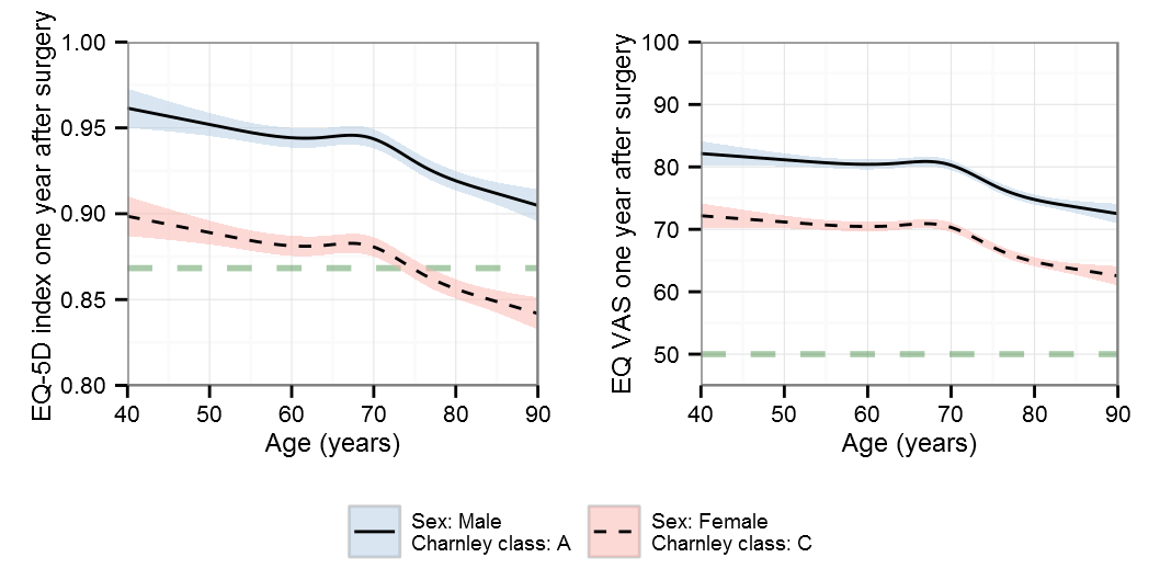
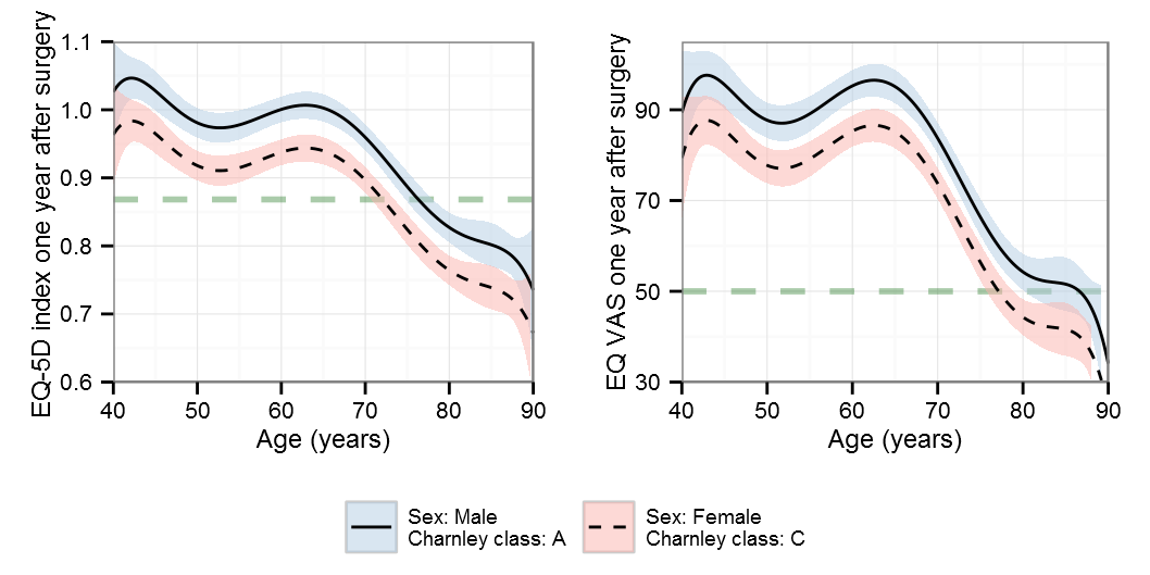
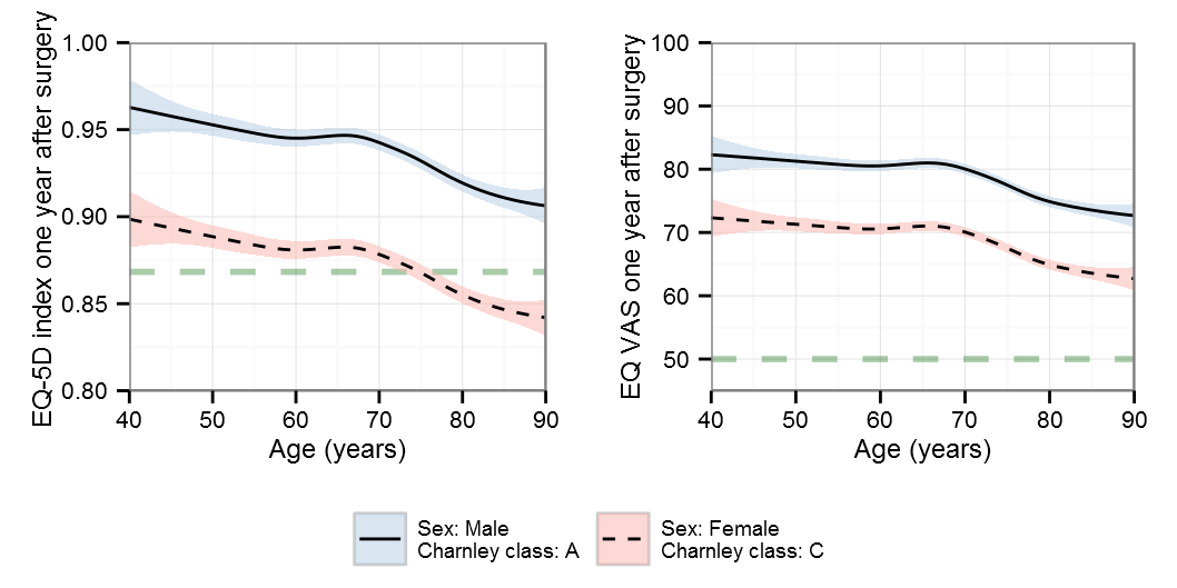
Restricted cubic splines
AIC
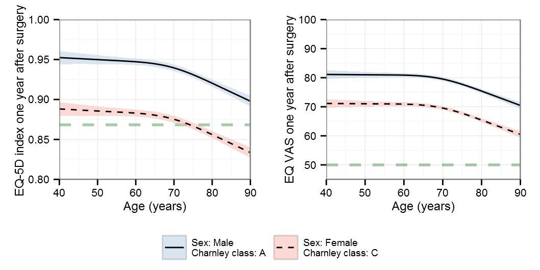
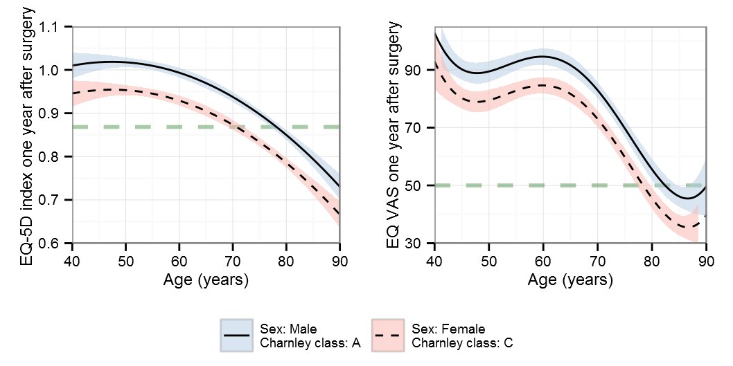
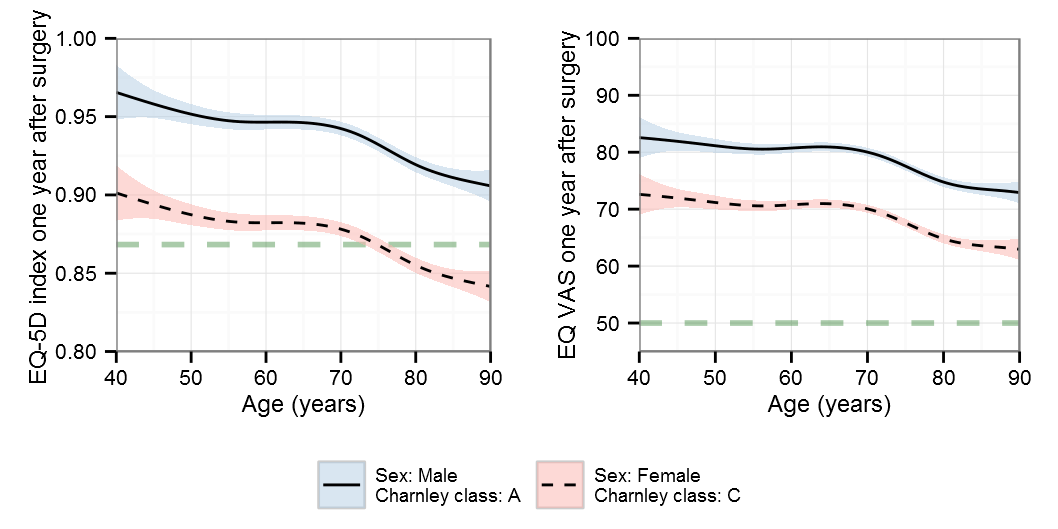
BIC
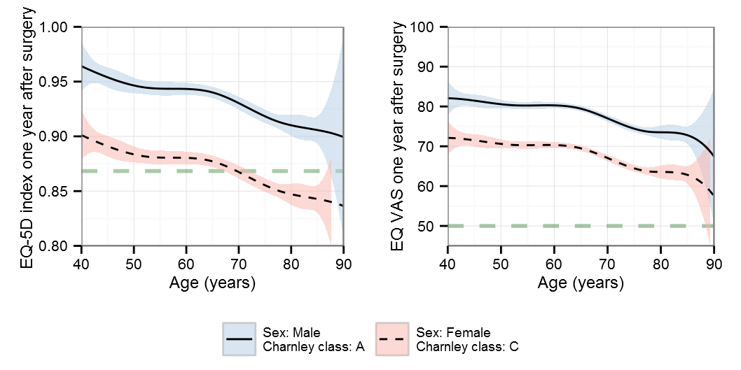
B-splines
AIC
BIC
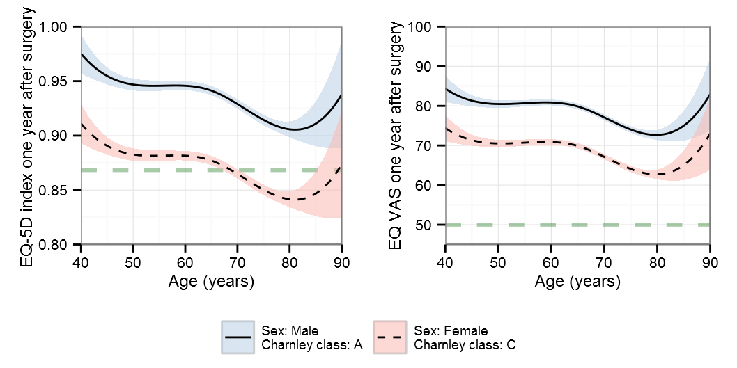
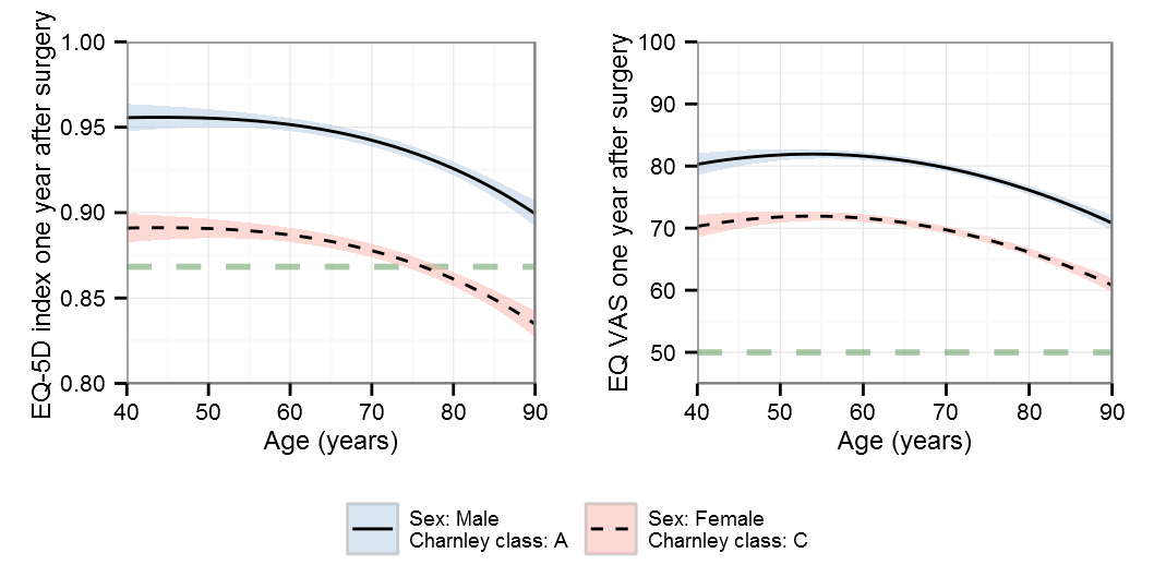
Polynomials
Note that the y-scale differs for the polynomials
AIC
BIC
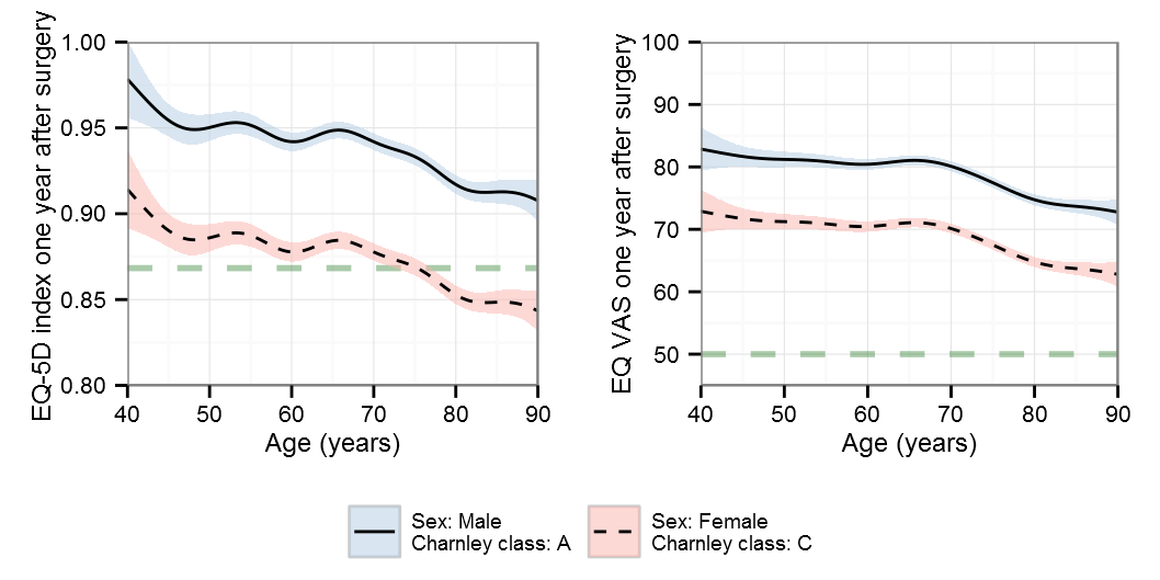
MFP – multiple fractional polynomial
Generalized additive models
Thin plate regression splines
Cubic regression splines
P-splines
Summary
I hope you enjoyed the post and found something useful. If there is some model that you lack, write up some code and I can see if it runs. Note that there are differences from the original supplement that used a slightly more complex setup for choosing the number of knots and a slightly different dataset.
Playing around with non-linearity
A friend just told me about amazing tool for playing around with splines, knots, etc that the Paul Lambert at the University of Leicester has created. I strongly recommend a visit to their site.
Hi,
Thank you for such an excellent article. I have one question.
For linear Regression Model the assumption is that the model is linear in the parameters (B0,B1) rather than in the predictors. Can you elaborate on this.
Regards,
Amit
Thanks! As an orthopaedic surgeon I’m probably not the best answer your question. There is an excellent Wikipedia article on the subject. You can also try CrossValidated, there best question on the subject that I’ve found is this one. Also have a look at John Fox’ nls appendix that contains some useful information.
Going back, the Wikipedia example is rather nice. If we translate it to the age and HRQoL setting we can see that βage*age may not be a good assumption. Although using the same transformation, βage 1*age/(βage 2 + age), makes little sense for age and HRQoL. We may instead try a model that more looks like βage 1*age-βage 2 * abs(age-βage 3) where we expect the βage 2 to be negative thus allowing for a ^ form where we expect a maximum and where the βage 3 may indicate where this occurs. The absolute value could of course be exchanged with a squared that may in turn provide a different estimate.
In my mind it seems that the nonlinear regression is best suited when you have simple relations defined by laws of nature such as the Michaelis–Menten kinetics. I believe that when working with more complex outcomes defining a sensible model is close to impossible although this could potentially be an alternative when you are trying to pinpoint the peak according to the previous formula.
I hope this gives some clarity, although keep in mind that I’m not a schooled statisticians and nonlinear regressions have never been a subject that I’ve been officially taught 😀
Hi Max
Thanks for sharing the code.
I was wondering if you could add some code for data simulation, the way one can pass it through the code and see how it works.
Many thanks beforehand.
Bye
Not sure of what you intend, I did have a question on CrossValidated where I simulate a non-linear dataset.
Thanks Max,
I just simply need the data.
I know you can not share your real data, what I ask is simulated data close to your original data.
All the best.
Sorry, but I can’t help you with this.