

As things change over time so should our statistical models. The image is CC by Prad Prathivi
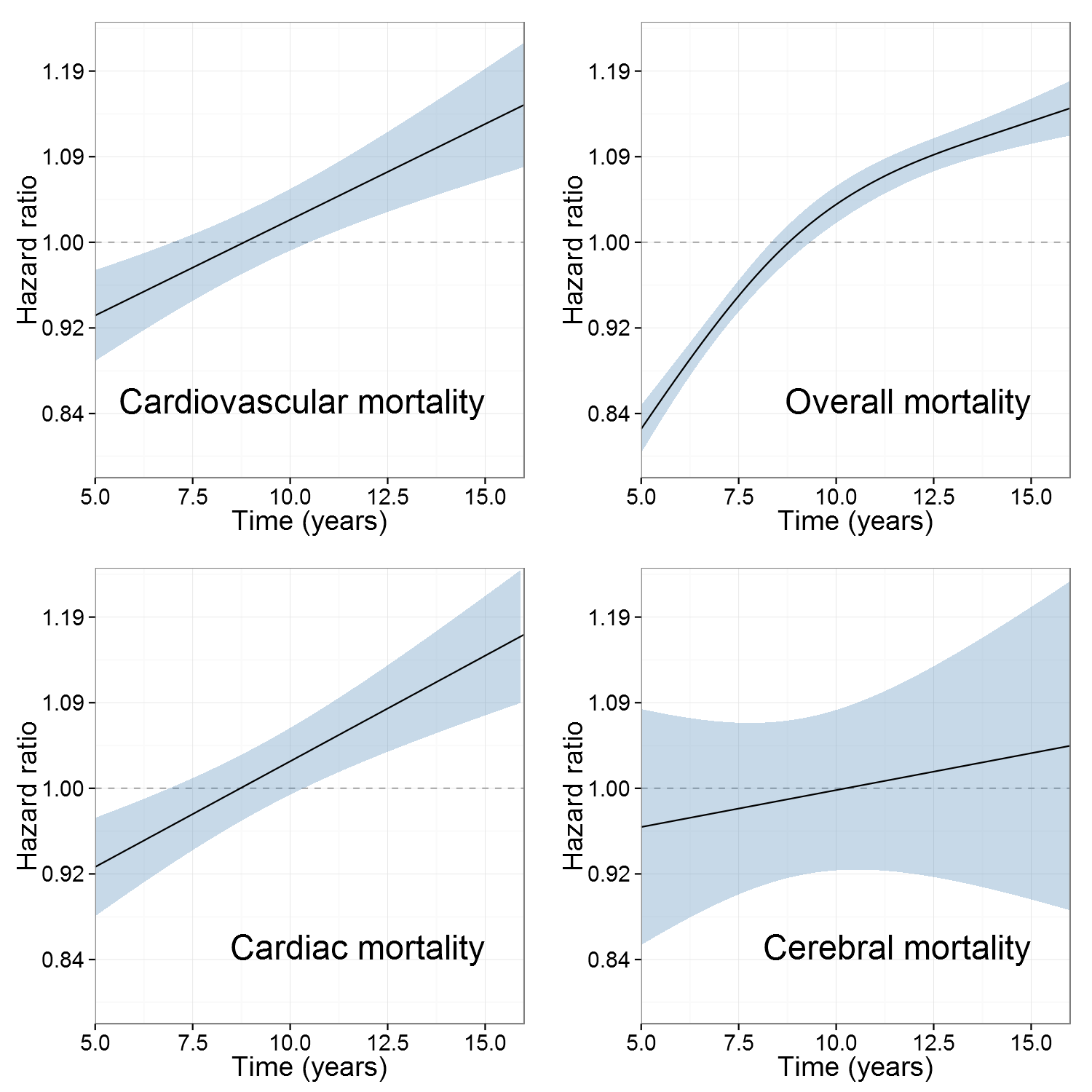
Since I’m frequently working with large datasets and survival data I often find that the proportional hazards assumption for the Cox regressions doesn’t hold. In my most recent study on cardiovascular deaths after total hip arthroplasty the coefficient was close to zero when looking at the period between 5 and 21 years after surgery. Grambsch and Thernau’s test for non-proportionality hinted though of a problem and as I explored it there was a clear correlation between mortality and hip arthroplasty surgery. The effect increased over time, just as we had originally thought, see below figure. In this post I’ll try to show how I handle with non-proportional hazards in R.
Why should we care?
As we scale up to larger datasets we are increasingly looking at smaller effects. This causes the models to become more susceptible to residual bias and problems in model assumptions.
Missing the exposure
In the example above I would have missed the fact that a hip implant may affect mortality in the long run. While the effect isn’t strong, it is one of the most frequent procedures and we have reasons to believe that subgroups may have an even higher risk of dying than the average patient with an hip implant.
Insufficient adjustment for confounding
If we assume that a variable is enough important to adjust for we also must accept that we should model it in optimal way so that all the confounding can’t affect our exposure variable.
What is the Cox model all about?
The key to understanding the Cox regression is grasping the concept of hazard. All regression models are basically trying to express (should be familiar from high-school):
[latex]y = A + B * X[/latex]
The core idea is that we can choose what we want to have as the y. Cox stated that if we assume that the proportion between hazards remains the same we can use the logarithm of the hazards function (h(t)) as the y:
[latex]h(t) = \frac{f(t)}{S(t)}[/latex]
Here the f(t) is the risk of dying at a certain moment in time while having survived that far, the S(t). In practice if we look at a certain moment we can estimate how many have made to that time point and then look at how many died at that particular point in time. An important resulting effect from this is that we can include a patient that appears after the study start and include that patient from that time point and onward. E.g. if Peter is operated with a hip arthroplasty in England, arrives after 1 year to Sweden, he has been alive for 1 year when we choose to include him. Note that any patient that would have died prior to that would never have come to our attention and we can therefore not include Peter in the S(t) when looking at the hazard prior to 1 year.
The start time is the key
The core idea of dealing with proportional hazards and time varying coefficients in a Cox model is to split the time and use an interaction term. We can do this similar to including Peter in the example above. We choose a suitable time interval and split all observations accordingly. If a patient is alive at the end of the interval he/she is simply marked as censored even if he/she eventually suffers an event. The advantage is that now we have a dataset where we have several starting times that we can use as interaction terms.
Important note: Always use the starting time and never the end time as the end time is invariably related to the event. Without time-splitting this is obvious as the interaction becomes highly significant and suddenly deviates sharply from the original estimate. If we have a more fine-grained time-split this becomes less of a problem but I still believe that it makes more sense in using the starting time as this should be completely free of all bias.
Splitting time with the Greg::timesplitter (R-code starts here)
My Greg-package (now on CRAN) contains a timeSplitter function that is a wrapper for the Epi package’s Lexis functionality. To illustrate how this works we start with 4 patients:
test_data <- data.frame(
  id = 1:4,
  time = c(4, 3.5, 1, 5),
  event = c("censored", "dead", "alive", "dead"),
  age = c(62.2, 55.3, 73.7, 46.3),
  date = as.Date(
    c("2003-01-01",
      "2010-04-01",
      "2013-09-20",
      "2002-02-23"))
)

test_data$time_str <- sprintf("0 to %.1f", test_data$time)
We can graph this using the grid package:
library(grid)
library(magrittr)
getMaxWidth <- function(vars){
  sapply(vars,
         USE.NAMES = FALSE,
         function(v){
           grobWidth(x = textGrob(v)) %>%
             convertX(unitTo = "mm")
         }) %>%
    max %>%
    unit("mm")
}
plotTitleAndPushVPs <- function(title_txt){
  pushViewport(viewport(width = unit(.9, "npc"),
                        height = unit(.9, "npc")))

  title <- textGrob(title_txt, gp = gpar(cex = 2))
  title_height <- grobHeight(title) %>%
    convertY(unitTo = "mm", valueOnly = TRUE) * 2 %>%
    unit("mm")
  grid.layout(nrow = 3,
              heights = unit.c(title_height,
                               unit(.1, "npc"),
                               unit(1, "npc") -
                                 title_height -
                                 unit(.1, "npc") -
                                 unit(2, "line"),
                               unit(2, "line"))) %>%
    viewport(layout = .) %>%
    pushViewport()
  viewport(layout.pos.row = 1) %>%
    pushViewport()
  grid.draw(title)
  upViewport()

  viewport(layout.pos.row = 3) %>%
    pushViewport()
}

plotLine <- function (row_no,
                      start_time,
                      stop_time,
                      event,
                      data_range = c(0, max(test_data$time)),
                      print_axis = FALSE) {
  viewport(layout.pos.row = row_no,
           layout.pos.col = 6,
           xscale = data_range) %>%
    pushViewport()
  on.exit(upViewport())

  if (event){
    grid.lines(x = unit(c(start_time,
                          stop_time), "native"),
               y = rep(0.5, 2))
    grid.points(x = unit(stop_time, "native"), y = 0.5,
                pch = "*",
                gp = gpar(cex = 2))
  }else{
    grid.lines(x = unit(c(start_time,
                          stop_time), "native"),
               y = rep(0.5, 2),
               arrow = arrow(length = unit(3, "mm"),
                             type = "closed"),
               gp = gpar(fill = "#000000"))
  }
  grid.points(x = unit(start_time, "native"), y = 0.5, pch = 20)
  if (print_axis)
    grid.xaxis()
}

plotIDcell <- function(row_no, id){
  viewport(layout.pos.row = row_no,
           layout.pos.col = 2) %>%
    pushViewport()
  grid.text(id)
  upViewport()
}
plotTimeStrcell <- function(row_no, time_str){
  viewport(layout.pos.row = row_no,
           layout.pos.col = 4) %>%
    pushViewport()
  grid.text(time_str)
  upViewport()
}

plotRowColor <- function(row_no, clr = "#F6F6FF"){
  viewport(layout.pos.row = row_no) %>%
    pushViewport()
  grid.rect(gp = gpar(col = clr, fill = clr))
  upViewport()
}


# Do the actual plot
grid.newpage()
plotTitleAndPushVPs("Time spans")
widths <-
  unit.c(unit(.1, "npc"),
         getMaxWidth(test_data$id),
         unit(.1, "npc"),
         getMaxWidth(test_data$time_str),
         unit(.1, "npc")) %>%
  unit.c(.,
         unit(1, "npc") - sum(.) - unit(.1, "npc"),
         unit(.1, "npc"))

grid.layout(nrow = nrow(test_data),
            ncol = length(widths),
            widths = widths) %>%
  viewport(layout = .) %>%
  pushViewport()


for (i in 1:nrow(test_data)){
  if (i %% 2 == 0)
    plotRowColor(i)
  plotIDcell(i, test_data$id[i])
  plotTimeStrcell(i, test_data$time_str[i])

  plotLine(row_no = i,
           start_time = 0,
           stop_time = test_data$time[i],
           event = test_data$event[i] == "dead",
           print_axis = i == nrow(test_data))
}
upViewport(2)
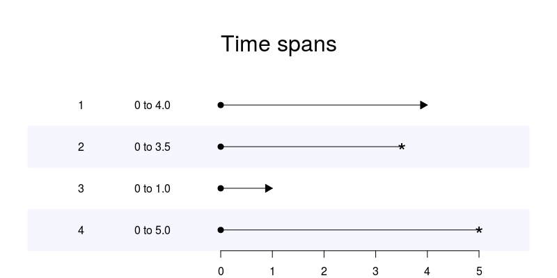
The * indicates events while the arrow are subjects that have been censored
Now we want to apply a split in 0.5 years:
library(Greg)
library(dplyr)
split_data <-
  test_data %>%
  select(id, event, time, age, date) %>%
  timeSplitter(by = 2, # The time that we want to split by
               event_var = "event",
               time_var = "time",
               event_start_status = "alive",
               time_related_vars = c("age", "date"))
plotTitleAndPushVPs("Time spans with split")

grid.layout(nrow = nrow(test_data) + nrow(split_data),
            ncol = length(widths),
            widths = widths) %>%
  viewport(layout = .) %>%
  pushViewport()

current_id <- NULL
no_ids <- 0
for (i in 1:nrow(split_data)){
  if (is.null(current_id) ||
      split_data$id[i] != current_id){
    current_id <- split_data$id[i]
    subjects_splits <- subset(split_data, id == current_id)
    rowspan <- (i + no_ids):(i + no_ids + nrow(subjects_splits))
    if (no_ids %% 2 == 1)
      plotRowColor(rowspan)
    plotIDcell(row_no = rowspan, id = current_id)
    plotTimeStrcell(row_no = rowspan, time_str = subset(test_data,
                                                        id == current_id,
                                                        "time_str"))
    with(subset(test_data,
                id == current_id),
         plotLine(row_no = i + no_ids,
                  start_time = 0,
                  stop_time = time,
                  event = event == "dead"))
    no_ids = no_ids + 1
  }

  plotLine(row_no = i + no_ids,
           start_time = split_data$Start_time[i],
           stop_time = split_data$Stop_time[i],
           event = split_data$event[i] == "dead",
           print_axis = i == nrow(split_data))
}
upViewport(2)
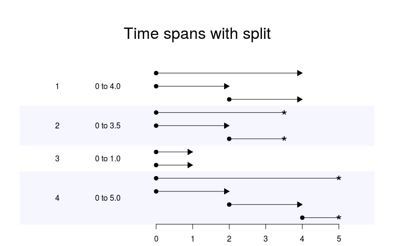
The * indicates events while the arrow are subjects that have been censored
Note that each subject has several time intervals where only the last interval contains the final status while all the previous are marked with a censored status. As you can see in the function call there is a time_related_vars argument where you provide other variables that need to be updated as we move forward in time (e.g. age).
Using the timeSplitter in our model
In order to illustrate this in a real Cox model we will use the melanoma dataset:
# First we start with loading the dataset
data("melanoma", package = "boot")

# Then we munge it according to ?boot::melanoma
library(dplyr)
library(magrittr)
melanoma %<>%
  mutate(status = factor(status,
                        levels = 1:3,
                        labels = c("Died from melanoma",
                                   "Alive",
                                   "Died from other causes")),
        ulcer = factor(ulcer,
                       levels = 0:1,
                       labels = c("Absent", "Present")),
        time = time/365.25, # All variables should be in the same time unit
        sex = factor(sex,
                     levels = 0:1,
                     labels = c("Female", "Male")))
Now we can fit a regular cox regression:
library(survival)
regular_model <- coxph(Surv(time, status == "Died from melanoma") ~
                         age + sex + year + thickness + ulcer,
                       data = melanoma,
                       x = TRUE, y = TRUE)
summary(regular_model)
Call:
coxph(formula = Surv(time, status == "Died from melanoma") ~
    age + sex + year + thickness + ulcer, data = melanoma, x = TRUE,
    y = TRUE)

  n= 205, number of events= 57

                  coef exp(coef)  se(coef)      z Pr(>|z|)
age           0.016805  1.016947  0.008578  1.959 0.050094 .
sexMale       0.448121  1.565368  0.266861  1.679 0.093107 .
year         -0.102566  0.902518  0.061007 -1.681 0.092719 .
thickness     0.100312  1.105516  0.038212  2.625 0.008660 **
ulcerPresent  1.194555  3.302087  0.309254  3.863 0.000112 ***
---
Signif. codes:  0 ‘***’ 0.001 ‘**’ 0.01 ‘*’ 0.05 ‘.’ 0.1 ‘ ’ 1

             exp(coef) exp(-coef) lower .95 upper .95
age             1.0169     0.9833    1.0000     1.034
sexMale         1.5654     0.6388    0.9278     2.641
year            0.9025     1.1080    0.8008     1.017
thickness       1.1055     0.9046    1.0257     1.191
ulcerPresent    3.3021     0.3028    1.8012     6.054

Concordance= 0.757  (se = 0.04 )
Rsquare= 0.195   (max possible= 0.937 )
Likelihood ratio test= 44.4  on 5 df,   p=1.922e-08
Wald test            = 40.89  on 5 df,   p=9.88e-08
Score (logrank) test = 48.14  on 5 df,   p=3.328e-09
If we do the same with a split dataset we get the exact same result (as it should be):
spl_melanoma <-
  melanoma %>%
  timeSplitter(by = .5,
               event_var = "status",
               event_start_status = "Alive",
               time_var = "time",
               time_related_vars = c("age", "year"))

interval_model <-
  update(regular_model,
         Surv(Start_time, Stop_time, status == "Died from melanoma") ~ .,
         data = spl_melanoma)

summary(interval_model)
Call:
coxph(formula = Surv(Start_time, Stop_time, status == "Died from melanoma") ~
    age + sex + year + thickness + ulcer, data = spl_melanoma,
    x = TRUE, y = TRUE)

  n= 2522, number of events= 57

                  coef exp(coef)  se(coef)      z Pr(>|z|)
age           0.016805  1.016947  0.008578  1.959 0.050094 .
sexMale       0.448121  1.565368  0.266861  1.679 0.093107 .
year         -0.102566  0.902518  0.061007 -1.681 0.092719 .
thickness     0.100312  1.105516  0.038212  2.625 0.008660 **
ulcerPresent  1.194555  3.302087  0.309254  3.863 0.000112 ***
---
Signif. codes:  0 ‘***’ 0.001 ‘**’ 0.01 ‘*’ 0.05 ‘.’ 0.1 ‘ ’ 1

             exp(coef) exp(-coef) lower .95 upper .95
age             1.0169     0.9833    1.0000     1.034
sexMale         1.5654     0.6388    0.9278     2.641
year            0.9025     1.1080    0.8008     1.017
thickness       1.1055     0.9046    1.0257     1.191
ulcerPresent    3.3021     0.3028    1.8012     6.054

Concordance= 0.757  (se = 0.04 )
Rsquare= 0.017   (max possible= 0.201 )
Likelihood ratio test= 44.4  on 5 df,   p=1.922e-08
Wald test            = 40.89  on 5 df,   p=9.88e-08
Score (logrank) test = 48.14  on 5 df,   p=3.328e-09
Now we can look for time varying coefficients using the survival::cox.zph() function:
cox.zph(regular_model) %>%
  extract2("table") %>%
  txtRound(digits = 2) %>%
  knitr::kable(align = "r")
| rho | chisq | p | |
|---|---|---|---|
| age | 0.18 | 2.48 | 0.12 |
| sexMale | -0.16 | 1.49 | 0.22 |
| year | 0.06 | 0.20 | 0.65 |
| thickness | -0.23 | 2.54 | 0.11 |
| ulcerPresent | -0.17 | 1.63 | 0.20 |
| GLOBAL | 10.30 | 0.07 |
The two variable that give a hint of time variation are age and thickness. It seems reasonable that melanoma thickness is less important as time increases, either the tumor was adequately removed or there was some remaining piece that caused the patient to die within a few years. We will therefore add a time interaction using the : variant (note using the * for interactions gives a separate variable for the time and that is not of interest in this case):
time_int_model <-
  update(interval_model,
         .~.+thickness:Start_time)
summary(time_int_model)
Call:
coxph(formula = Surv(Start_time, Stop_time, status == "Died from melanoma") ~
    age + sex + year + thickness + ulcer + thickness:Start_time,
    data = spl_melanoma, x = TRUE, y = TRUE)

  n= 2522, number of events= 57

                          coef exp(coef)  se(coef)      z Pr(>|z|)
age                   0.014126  1.014226  0.008591  1.644 0.100115
sexMale               0.511881  1.668427  0.268960  1.903 0.057016 .
year                 -0.098459  0.906233  0.061241 -1.608 0.107896
thickness             0.209025  1.232476  0.061820  3.381 0.000722 ***
ulcerPresent          1.286214  3.619060  0.313838  4.098 4.16e-05 ***
thickness:Start_time -0.045630  0.955395  0.022909 -1.992 0.046388 *
---
Signif. codes:  0 ‘***’ 0.001 ‘**’ 0.01 ‘*’ 0.05 ‘.’ 0.1 ‘ ’ 1

                     exp(coef) exp(-coef) lower .95 upper .95
age                     1.0142     0.9860    0.9973    1.0314
sexMale                 1.6684     0.5994    0.9848    2.8265
year                    0.9062     1.1035    0.8037    1.0218
thickness               1.2325     0.8114    1.0918    1.3912
ulcerPresent            3.6191     0.2763    1.9564    6.6948
thickness:Start_time    0.9554     1.0467    0.9134    0.9993

Concordance= 0.762  (se = 0.04 )
Rsquare= 0.019   (max possible= 0.201 )
Likelihood ratio test= 48.96  on 6 df,   p=7.608e-09
Wald test            = 45.28  on 6 df,   p=4.121e-08
Score (logrank) test = 56.29  on 6 df,   p=2.541e-10
If you want to extend this for non-linearity it requires some additional tweaking, see the vignette in the package for more details. A tip is to use the rms package’s contrast function as you start working on your graphs. Note that the rms::cph has issues handling the time interaction effect and you therefore need to create your a new time interaction variable in the dataset before doing the regression, i.e.:
# The survival model
library(survival)
coxph(Surv(start_time, end_time, event) ~ var1 + var2 + var2:start_time, data=my_data)

# Must be converted to this
my_data$var2_time = var2*start_time
cph(Surv(start_time, end_time, event) ~ var1 + var2 + var2_time, data=my_data)

# If the variable is a factor, e.g. smoking
my_data$smoking_time = (smoking == "Yes")*start_time
cph(Surv(start_time, end_time, event) ~ var1 + smoking + smoking_time, data=my_data)
Why not use survival::tt()?
The survival package has a way of dealing with this that is to use the the tt() function together with the tt argument. While this is an excellent strategy it often doesn’t work with large datasets as its time-split is too fine grained (if I’ve understood it correctly). You can though find an excellent vignette on how to apply it here.
Using the timereg package
I’ve tried to use the timereg package but I haven’t figured out how to get smooth splines over time. The documentation is also sparse without any illustrative vignette.
Time-split and memory limitations
Drop unused variables
If you find that you’re running out of memory make sure to drop any variables that you aren’t using in your model. It also seems to speed up the regression so its seems like a good rule of thumb to only keep the variables you really want once you start modeling.
Length of time interval
I’ve frequently used 0.5 years as the time-split interval. This as the cox.zph then no longer indicates non-proportionality while the dataset doesn’t explode too much for my computer to handle. I think the underlying biological process can help you guess suitable time intervals.
Using strata()
If you have a confounder that indicates a non-proportional hazard a valid approach is to set that variable as a strata. Note that this is not possible with continuous variables or if one strata is too small for evaluating the full model within that strata.
Summary
In summary you need to split your data into time intervals and then use the starting time as an interaction term using the :. The Greg package helps with the technical details of generating the data. I hope you found this solution both intuitive and useful.
Thanks for the nice documentation. I was wondering if the timeSplitter function works also with interval-censored data like in the survSplit-function?
Hi Max! This is very interesting. Do you happen to have code on how you made the first plots (http://gforge.se/wp-content/uploads/2016/03/Time_hzrd_spline-1.png)?
Dear Max, I was able to pass the proportionality test with cox.zph using your suggestion. How do I cite you? I split the time with manual codes, but follow your suggestion on tstart*variable interaction.
However, my time interaction variables seem to have significant effect statistically, but the substantial effects (i.e. exp(coef) became 1 or very close to that. Your result for thickness:Start_time is also very close to 1. Is this to be expected? What’s the interpretation of this? Should we be concerned? My 4 interaction variables are 1.0004, 0.9996, 1.0003 and 0.9994… so I am a little puzzled.
Sorry for the late reply, I sometimes don’t get the WP notifications of new comments 🙁
Regarding your question it is a little hard to fully grasp. I assume that the time interacts with your main variable of interest and thus you need to look at them both in order to fully grasp what is going on. I usually do a plot. If your interaction variable is really tiny and you can’t see it in a plot it is hard to understand why the PH assumption was broken in the first place.
Regarding citing I used the methodology for the first time (if I remember correctly) in this article 10.1097/MD.0000000000002662