The new rmarkdown revolution has started. The image is CC by Jonathan Cohen.

The new R Markdown (rmarkdown-package) introduced in Rstudio 0.98.978 provides some neat features by combining the awesome knitr-package and the pandoc-system. The system allows for some neat simplifications of the fast-track-publishing (ftp) idea using so called formats. I’ve created a new package, the Grmd-package, with an extension to the html_document format, called the docx_document. The formatter allows an almost pain-free preparing of MS Word compatible web-pages.

In this post I’ll (1) give a tutorial on how to use the docx_document, (2) go behind the scenes of the new rmarkdown-package and RStudio ≥ 0.98.978, (3) show what problems currently exists when skipping some of the steps outlined in the tutorial.

Tutorial on how to use ftp with the rmarkdown implementation

A major improvement in the new rmarkdown is the YAML set-up. It is now much easier to set-up environments for your documents, all you need to look at is the function arguments in the documentation and provide those in the file. You have four different default document types where some options shared while other are output-specific: html_document, pdf_document, word_document, or markdown_document.

As mentioned above, the Grmd-package also contains a formatter, the docx_document format that is a wrapper around the html_document. It has the same options as the html_document with a few additions/defaults adapted to the concept of fast-track-publishing. As the package depends on rmarkdown it can currently only installed from Github (CRAN does not allow dependencies on packages outside CRAN) and in order to install the package you need to use the devtools-package:

# If you don't have devtools install run below line:
install("devtools")
# Then install the Grmd-package by running below code:
devtools::install_github("gforge/Grmd")

After this you simply put at the top of your Rmd-document:

---
output: Grmd::docx_document
---

If you may notice that after adding the above change from html_document to the custom Gmisc::docx_document-format the choice knit-box intelligently changes from:

to:

As RStudio is uncertain of how to approach this new format. Note: interestingly this also occurs if you happen to set the rstudio.mardownToHTML option using options().

For this tutorial we will use the Rmd document found in the Github ftp-repository. It is a simple example using my two main packages. Thus the new Rmd file is:

---
title: "A fast-track-publishing demo"
output: 
  Grmd::docx_document:
    fig_caption: TRUE
    force_captions: TRUE
---

End section of methods
======================

```{r Data_prep, echo=FALSE, message=FALSE, warning=FALSE}
# Moved this outside the document for easy of reading
# I often have those sections in here
source("Setup_and_munge.R")
```

```{r Versions}
info <- sessionInfo()
r_ver <- paste(info$R.version$major, info$R.version$minor, sep=".")
```

All analyses were performed using R (ver. `r r_ver`)[R Core Team, 2013] and packages rms (ver. `r info$otherPkgs$rms$Version`) [F. Harrell, 2014] for analysis, Gmisc for plot and table output (ver. `r info$otherPkgs$Gmisc$Version`), and knitr (ver `r info$otherPkgs$knitr$Version`) [Xie, 2013] for reproducible research.

Results
=======

We found `r nrow(melanoma)` patients with malignant melanoma between the years `r paste(range(melanoma$year), collapse=" and ")`. Patients were followed until the end of 1977, the median follow-up time was `r sprintf("%.1f", median(melanoma$time_years))` years (range `r paste(sprintf("%.1f", range(melanoma$time_years)), collapse=" to ")` years). Males were more common than females and had also a higher mortality rate.

```{r Table1, cache=FALSE}
table_data <- list()
getT1Stat <- function(varname, digits=0){
  getDescriptionStatsBy(melanoma[, varname], melanoma$status, 
                        add_total_col=TRUE,
                        show_all_values=TRUE, 
                        hrzl_prop=TRUE,
                        statistics=FALSE, 
                        html=TRUE, 
                        digits=digits)
}

# Get the basic stats
table_data[["Sex"]] <- getT1Stat("sex")
table_data[["Age†"]] <- getT1Stat("age")
table_data[["Ulceration"]] <- getT1Stat("ulcer")
table_data[["Thickness‡"]] <- getT1Stat("thickness", digits=1)

mergeDesc(table_data) %>%
  htmlTable(header = gsub("[ ]*death", "", colnames(table_data[[1]])),
            # Add a column spanner
            cgroup = c("", "Death"),
            n.cgroup = c(2, 2),
            caption="Baseline characteristics", 
            tfoot="† Age at the time of surgery.
            ‡ Tumour thickness, also known as Breslow thickness, measured in mm.",
            align="rrrr",
            css.rgroup = "")

```

Main results
------------

```{r C_and_A, results='asis'}
label(melanoma$sex) <- "Sex"
label(melanoma$age) <- "Age"
label(melanoma$ulcer) <- "Ulceration"
label(melanoma$thickness) <- "Breslow thickness"

# Setup needed for the rms coxph wrapper
ddist <- datadist(melanoma)
options(datadist = "ddist")

# Do the cox regression model 
# for melanoma specific death
msurv <- Surv(melanoma$time_years, melanoma$status=="Melanoma death")
fit <- cph(msurv ~ sex + age + ulcer + thickness, data=melanoma)

# Print the model
printCrudeAndAdjustedModel(fit, 
                           desc_digits=0,
                           caption="Adjusted and unadjusted estimates for melanoma specific death.",
                           desc_column=TRUE,
                           add_references=TRUE, 
                           ctable=TRUE)

pvalues <- 
  1 - pchisq(coef(fit)^2/diag(vcov(fit)), df=1)
```

After adjusting for the three variables, age, sex, tumor thickness and ulceration, only the latter two remained significant (p-value `r txtPval(pvalues["ulcer=Present"], lim.sig=10^-3)` and `r txtPval(pvalues["thickness"], lim.sig=10^-3)`), see table `r as.numeric(options("table_counter"))-1` and Fig. `r figCapNoNext()`.

```{r Regression_forestplot, fig.height=3, fig.width=5, out.height=300, out.width=500, dpi=300, fig.cap=figCapNo("A forest plot comparing the regression coefficients.")}
# The output size can be fixed by out.width=625, out.height=375 but you loose the caption
# I've adjusted the coefficient for age to be by 
forestplotRegrObj(update(fit, .~.-age+I(age/10)), 
                  order.regexps=c("Female", "age", "ulc", "thi"),
                  box.default.size=.25, xlog=TRUE, zero=1,
                  new_page=TRUE, clip=c(.5, 6), rowname.fn=function(x){
  if (grepl("Female", x))
    return("Female")
  
  if (grepl("Present", x))
    return("Ulceration")
  
  if (grepl("age", x))
    return("Age/10 years")

  return(capitalize(x))
})
```

```

with the accompanying setup_and_munge.R script:

##################
# Knitr settings #
##################

knitr::opts_chunk$set(warning=FALSE,
                      message=FALSE,
                      echo=FALSE,
                      dpi=96,
                      fig.width=4, fig.height=4, # Default figure widths
                      dev="png", dev.args=list(type="cairo"), # The png device
                      # Change to dev="postscript" if you want the EPS-files
                      # for submitting. Also remove the dev.args() as the postscript
                      # doesn't accept the type="cairo" argument.
                      error=FALSE)

# Evaluate the figure caption after the plot
knitr::opts_knit$set(eval.after='fig.cap')

# Use the table counter that the htmlTable() provides
options(table_counter = TRUE)

# Use the figCapNo() with roman letters
options(fig_caption_no_roman = TRUE)

#################
# Load_packages #
#################
library(rms) # I use the cox regression from this package
library(boot) # The melanoma data set is used in this exampe
library(Gmisc) # Stuff I find convenient
library(Greg) # You need to get this from my GitHub see http://gforge.se/Gmisc
library(magrittr) # The excellent piping package

##################
# Munge the data #
##################

# Here we go through and setup the variables so that
# they are in the proper format for the actual output

# Load the dataset - usually you would use read.csv
# or something similar
data("melanoma")

# Set time to years instead of days
melanoma$time_years <-
  melanoma$time / 365.25

# Factor the basic variables that
# we're interested in
melanoma$status <-
  factor(melanoma$status,
         levels=c(2, 1, 3),
         labels=c("Alive", # Reference
                  "Melanoma death",
                  "Non-melanoma death"))
melanoma$sex <-
  factor(melanoma$sex,
         labels=c("Male", # Reference
                  "Female"))

melanoma$ulcer <-
  factor(melanoma$ulcer,
         levels=0:1,
         labels=c("Absent", # Reference
                  "Present"))

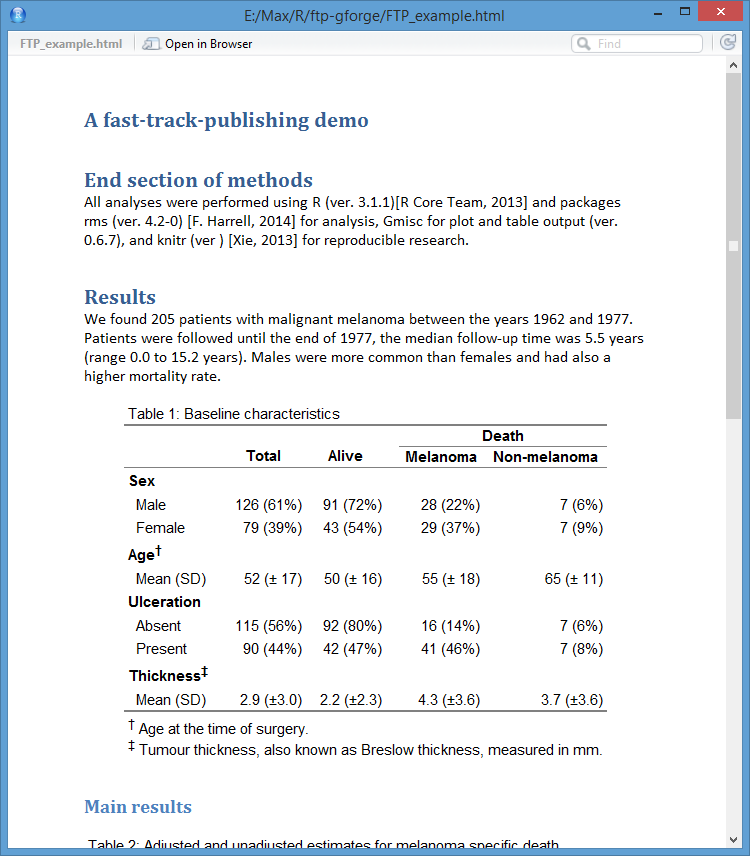
Will provide the following browser output:

Copy-paste directly from browser

Copy-pasting directly from the web-browser works! The current compatibility that I've checked are (Windows 8.1):

• RStudio viewer ≤ 0.98.978: works for headers, text, and tables but not for images.
• Internet explorer ≥ v.11: works for all (headers, text, tables, and images).
• Chrome ≥ v.36: works for all (headers, text, tables, and images).
• Firefox ≤ v.31: works for no elements.

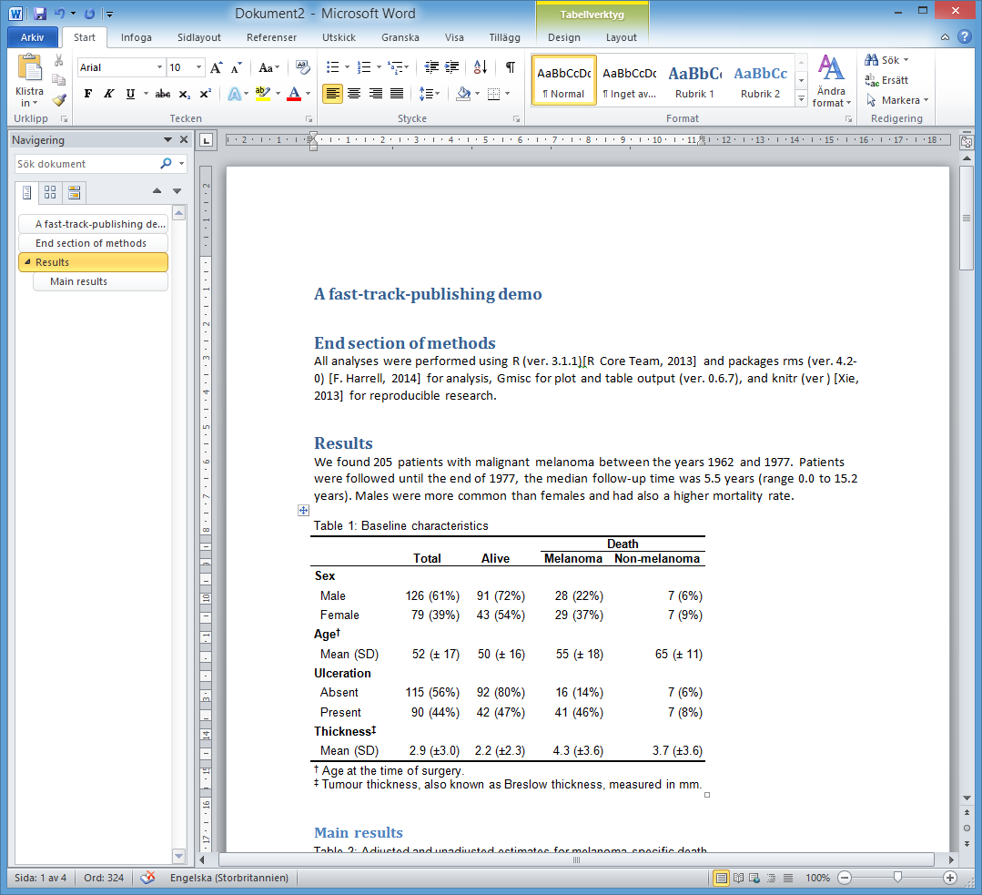
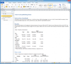
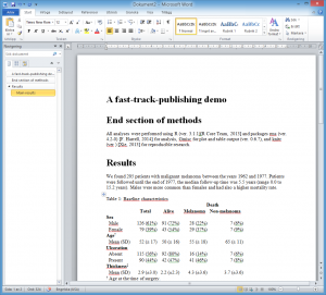
Just choose a compatible browser from the above list, open the .html-file, select everything, copy->paste it directly into Word, and you'll get the following beauty:

The end result in MS Word

Go through LibreOffice

Going through LibreOffice will produce a very similar result to the above but you will additionally also have the image at the bottom (that is if you are not copy-pasting from Chrome/IE).

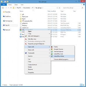
To open the file, navigate to it using the explorer, right click on the html-file and open it in LibreOffice as below (click on the image to enlarge):

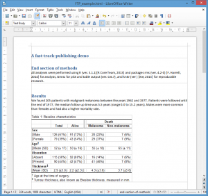
And you will get the following:

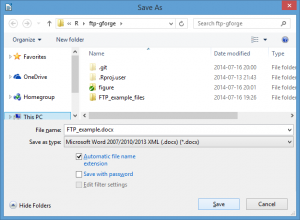
Staying here and working in LibreOffice is probably an excellent alternative but if you still want the .docx-file for MS Word then go to File > Save As.. (or press Ctrl+Shift+S) and choose the .docx format as below:

Now simply open the .docx-file in Word

I hope you found this tutorial useful and good luck with getting your masterpiece published!

Behind the scenes with the rmarkdown-package and RStudio

The R markdown v2 took some time getting used to. One of the first changes was that the environment no longer includes the knitr-package. To access the knitr options we now have to either include the package manually or use the :: operator. E.g. when setting the knitr chunk options:

knitr::opts_chunk$set(
  warning=FALSE,
  message=FALSE,
  echo=FALSE,
  dpi=96,
  fig.width=4, fig.height=4, # Default figure widths
  dev="png", dev.args=list(type="cairo"), # The png device
  # Change to dev="postscript" if you want the EPS-files
  # for submitting. Also remove the dev.args() as the postscript
  # doesn't accept the type="cairo" argument.
  error=FALSE
)

As LibreOffice ignores some of the formatting presented in the CSS the current alternative is to specify at the element-level the option through post-processing the html-document. This was actually a little tricky to figure out, the rmarkdown runs the render() function that has the option of applying a post-processor to the output. Unfortunately this can not be provided to the html_document as this has it's own post-processor that it attaches to the output_format object. As I didn't want to replace the default post-processor with my own, I needed to write a rather complex formatter that runs the new post-processor after the first, hence core of the docx_document() formatter does this (the actual code also does some additional cleaning):

# Gets the output_format
output_ret_val$post_processor_old <-
  output_ret_val$post_processor

# Wraps the old with the new post-processor
output_ret_val$post_processor <-
  post_processor <- function(metadata, input_file, output_file, clean, verbose,
                             old_post_processor =  output_ret_val$post_processor_old) {
    # Call the original post-processor in order to limit the changes that this function
    # has on the original functionality
    output_file <-
      old_post_processor(
        metadata = metadata,
        input_file = input_file,
        output_file = output_file,
        clean = clean,
        verbose = verbose
      )
    
    # read the output file
    output_str <- readLines(output_file, warn = FALSE, encoding = "UTF-8")
    
    # Annoyingly it seems that Libre Office currently
    # 'forgets' the margin properties of the headers,
    # we therefore substitute these with a element specific
    # style option that works. Perhaps not that pretty but
    # it works and can be tweaked for most things.
    output_str <-
      gsub(
        paste0(''),
        paste0(''),
        gsub(
          paste0(''),
          paste0(''),
          output_str
        )
      )
    
    writeLines(output_str, output_file, useBytes = TRUE)
    return(output_file)
  }

Dealing with high-resolution images

High-resolution images (DPI ≥ 300) are frequently needed for press. As in the example you need to specify the dip=300 in the knitr-chunk. Doing this will unfortunately blow upp the image to an uncomfortable large size and it may be therefore interesting limiting the screen output size. For this you use the out.width and the out.height. Since these elements are not available in markdown knitr inserts a plain <img src="..." /> element without captions. To remedy this you can set force_captions=true as in the example. It will use the XML package and replace <p><img .../></p> with an element identical to the pandoc image with caption (see the function that is invoked by docx_document below).

prCaptionFix <- function(outFile){
  # Encapsulate within a try since there is a high risk of unexpected errors
  tryCatch({
    # Open and read the file generated by pandoc
    tmp <- XML::htmlParse(outFile, encoding="utf-8", replaceEntities = FALSE)

    # The caption-less images are currently located under a p-element instead of a div
    caption_less_images <- xpathApply(tmp, "/html/body//p/img")
    for (i in 1:length(caption_less_images)){
      old_node <- xmlParent(caption_less_images[[i]])
      img_clone <- xmlClone(caption_less_images[[i]])
      new_node <- newXMLNode("div",
                             img_clone,
                             newXMLNode("p",
                                        xmlAttrs(img_clone)["title"],
                                        attrs=c(class="caption")),
                             attrs=c(class="figure"))
      replaceNodes(oldNode = old_node,
                   newNode = new_node)
    }

    saveXML(tmp, encoding = "utf-8", file=outFile)
  }, error=function(err)warning("Could not force captions - error occurred: '", err, "'"))

  return(outFile)
}

A few minor RStudio-tips

For those of you developing packages in RStudio, here are some neat functions that I currently like (not specific to the latest version):

• Ctrl+Shift+L Calls the devtools::load_all(".") from within a package. This gives you access to all the private functions and is much faster than rebuilding the full package. Note: if you haven't installed the package the key combination does not work and you won't even get an error.
• Ctrl+Shift+T Runs the package tests.
• Ctrl+Alt+left/right arow Quickly switches between tabs.
• Ctrl+Shift+F find in all files, very handy for navigating.

Issues that the current solution resolves

I've gotten quite a lot of response to the ftp-concept, especially now that the new functionality that caused some new bugs to appear with the old ftp-approach. In this section we'll look a little at what happens when skipping some of the steps.

Direct pandoc Word output

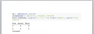
I believe that this will be the future but unfortunately pandoc's table abilities lacks the finesse that I like. In order to get reviewers quickly acquainted with the study results I think that nice tables can't hurt. E.g. the table below is far from satisfactory in my opinion:

---
output: word_document
---

```{r, results='asis'}
mx <- matrix(1:6, ncol=3)
colnames(mx) <- c("First", "Second", "Third")
knitr::kable(mx, align=c("l", "c", "r"), format="pandoc", caption="Test table")
```

Opening html in Word

Importing html-documents into Word has for some unknown reason not been a priority for the Microsoft developers. I'm surprised that the import isn't more advanced more than two decades since the web began. Currently the major problem is that you loose the table cell borders:

Opening in LibreOffice and copy-pasting from there

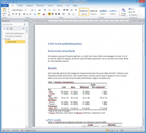
Somewhat odd that this doesn't work. When copy-pasting from LibreOffice to Word the formatting of the headers suddenly end up with a 14pt margin below, see below image:

Opening in Firefox and copy-pasting into Word

As you see below, most of the formatting is lost when using this approach: