Cool woven artwork on the campus of Kansas University. The image is CC by Patrick Emerson

I recently started to work with Sweave (by Friedrich Leisch) and found it a truly awesome package. The ease of use is amazing. In this post I’ll try to get you started with first Sweave and then the knitr (by Yihui Xie). The knitr package is a more advanced version of Sweave, update: Start with knitr as it’s really well integrated into RStudio and is more actively developed.

Reasons for learning LaTeX & Sweave/knitr:

• You can export formatted tables (ready for publication)
• You connect the results with the actual calculations, minimizing risk of “copy->paste” errors
• The code is “automatically documented” as you explain the results in the text
• You can easily re-run the report on a new dataset

Now lets get started…

Install & setup LaTeX/TeX

First, install the TeX software to be able to create the PDF. I use MiKTeX – probably the most commonly used TeX implementation for Windows. You can find it here.

LaTeX is a old typesetting language (TeX started in 1977, LaTeX is just a version of TeX with collections of pre-built macros) that allows you to write advanced formulas etc in plain text and then getting beautiful PDF:s. You need some basic LaTeX skills to get work with Sweave, you can find some good help here:

• David R. Wilkins has a nice introduction to LaTeX.
• A more intro advanced for the Harvard math dep. Detailed but good if you want to dig in deeper
• An excellent forum for LaTeX is Stackoverflow’s TeX- LaTeX.

To edit my LaTeX files I use WinShell, it’s free and you can find it here.

A very basic example of a LaTeX file can look like this:

\documentclass[10pt,a4paper]{article}
\begin{document}

My awesome \LaTeX test

\end{document}

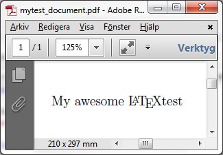
That compiles into this PDF (press F11 in WinShell):

Notice that the file name ends with a .tex and that I use _ instead of whitespace in the file name. You can run into problems with whitespaces and it’s therefore best to avoid them although in most of the cases it will work fine (ie not mytest document.tex but mytest_document.tex)

 Sweave – weave S into LaTeX

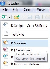
The Sweave package is fairly easy to get started with, especially in RStudio. All you need to do is create a Sweave document:

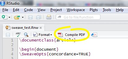
Then click on the Compile PDF-button. You have to save the file to be able to compile it, remember to leave out the whitespaces and the file ending should be .Rnw:

Now to add some R to the document I use the:

<<name, options>>=
R-code
@

to put in blocks of code. The name is an easy way to say what that part is doing so that you quickly can find it if you’ve folded the code block (press the tiny arrow to the left of the code, next to the line number).

Now I’ve added some stuff to the previous example:

\documentclass{article}

\begin{document}
\SweaveOpts{concordance=TRUE}

My awesome \LaTeX test

<<Test, echo=TRUE, results=verbatim>>=
variable1 <- 1
variable2 = 2
hello_txt <- "Hello world" # just to illustrate the markup
@

I've now created two variables, one with the value \Sexpr{variable1}
and one with the value \Sexpr{variable2}. I've used two different 
assignment operators, the $<-$ and the $=$. The $<-$ is preferred because 
it gives a natural understanding of assignment since the $<-$ looks 
like an arrow while $=$ can be confused with equal (that usually 
is represented by two equal signs "$==$").

We can reference the variable a a little further down:

<<Add the variables, echo=FALSE, results=verbatim>>=
variable1 + variable2
print(hello_txt)
@

Thats all!

\end{document}

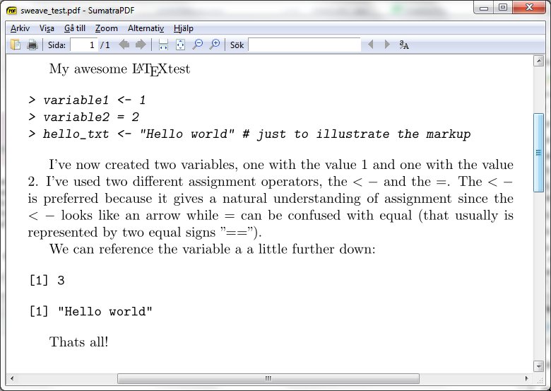
The output is:

Now this was a very simple example but you can as advanced as you want.

Troubleshooting Sweave

Here are some of the issues and the solutions that I’ve had when learning Sweave.

If you try to run the Sweave tex file in WinShell (note: RStudio creates a .tex file from the .Rnw file that is plain LaTeX where the R code has been translated. It resides in the same directory as the .Rnw file) you may get a complaint that Sweave.sty is not found. If you get this just add under the Windows controle panel -> System -> Advanced settings a new environment variable called TEXINPUT with the directory containing the Sweave.sty (you can search for it, in my case it’s: “C:\Software\R\R-2.15.0\share\texmf\tex\latex”).

Stuff that sometimes causes me issues is the \hbox overfull message in tables. I’ve sometimes solved this by editing the TeX code in WinShell, limiting the text in the or getting a multiline cell but I’ve also used the geometry package in some parts:

\newgeometry{textwidth=18cm}
... my very wide table ...
\restoregeometry

Important note: All your code has to be in the Sweave document since it runs in it’s own environment in R. You can check your code without creating a PDF by pressing Ctrl+Alt+R. You can run just a block of code by pressing Ctrl+Alt+C. The options are available in the top right of the RStudio editor.

knitr – knitting R into LaTeX

Make sure that all your packages are up to date:

update.packages(ask = FALSE)

Now you install the knitr package and all it’s dependencies:

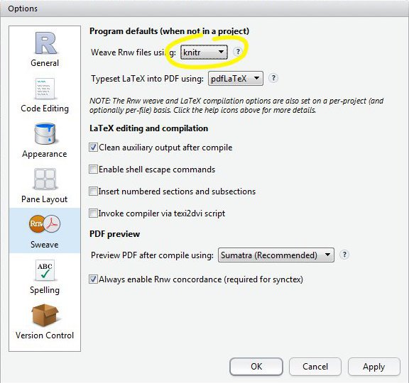
install.packages("knitr", dependencies=TRUE)

Change the Sweave environment to knitr, in Tools -> Options menu:

There are a few differences to the code above, basically you have some other results options that I’ve changed:

\documentclass{article}

\usepackage{graphicx, color, framed, alltt}

\begin{document}

My awesome \LaTeX test

<<label="Test", results='markup'>>=
variable1 <- 1
variable2 = 2
hello_txt <- "Hello world" # just to illustrate the markup
@

I've now created two variables, one with the value \Sexpr{variable1}
and one with the value \Sexpr{variable2}. I've used two different 
assignment operators, the $<-$ and the $=$. The $<-$ is preferred because 
it gives a natural understanding of assignment since the $<-$ looks 
like an arrow while $=$ can be confused with equal (that usually 
is represented by two equal signs "$==$"). 

We can reference the variable a a little further down:

<<label="Add the variables", echo=FALSE, results='markup'>>=
variable1 + variable2
print(hello_txt)
@

Thats all!

\end{document}

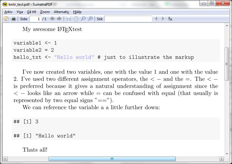
With the output:

You get basically the same as you did with Sweave but with a nicer R-output. There are a lot of new features with knitr that I haven’t covered and I’m planning on getting back to this topic once I learn more.

There are a lot of very nice web-resources on knitr:

• Jeromy Anglim has a nice post about converting a Sweave document to knitr
• Yihui Xie has also a very helpful post about knitr and Sweave

Troubleshooting knitr

I actually didn’t have that many issues with the transition as I was afraid at the start.

One thing that I noticed was that I had to install the Rcpp separately and it also complained in R 2.15.0 – I had to update to 2.15.1 to get it working:

install.packages(“Rcpp”)

Jeromy Anglim has a some good posts about knitr, check our his Sweave to knitr post

The future?

Although I really like LaTeX it is a little cumbersome to convert into Word. I usually use TeX4ht (htla­tex) to convert to HTML. It works fine, although the tables need minor fixing. I’m thinking about converting to Markdown, especially since I recently learned that the pictures get embedded in the HTML document and not as separate files… We’ll see if I’ll get back to this in a future post.